0x560 Model

1. Vocoder
- 1.1. AR Vocoder
- 1.2. NAR Vocoder
2. Acoustic Model
3. Alignment

1. Vocoder

Vocoder takes the acoustic features (mel spectrogram or discrete ids) into a time-domain audio waveform.

This Youtube is a very good summary of neural vocoder

1.1. AR Vocoder

Model (WaveNet)

Use stack of dilated causal convolution layer to increase receptive field

\(\mu\)-law is applied to quantize 16bit to 8bit representation to enable softmax

\[f(x) = sign(x)\frac{\ln (1+\mu|x|)}{1+\mu}\]

It is using gated activation unit as the nonlinearity

\[z = \tanh(W_f * x) \odot \sigma(W_g * x)\]

When it is conditional on some inputs \(h\), it becomes

\[z = \tanh(W_f * x + V_f^Th) \odot \sigma(W_g * x + V_g^h)\]

The condition on \(h\) can be either global or local.

when it is a glocal condition, \(h\) is broadcast
When it is a local condition, \(h\) is upsampled to match the resolution

Model (FFTNet)

Achieves dilation effect by splitting the input into two parts

Model (WaveRNN)

1.2. NAR Vocoder

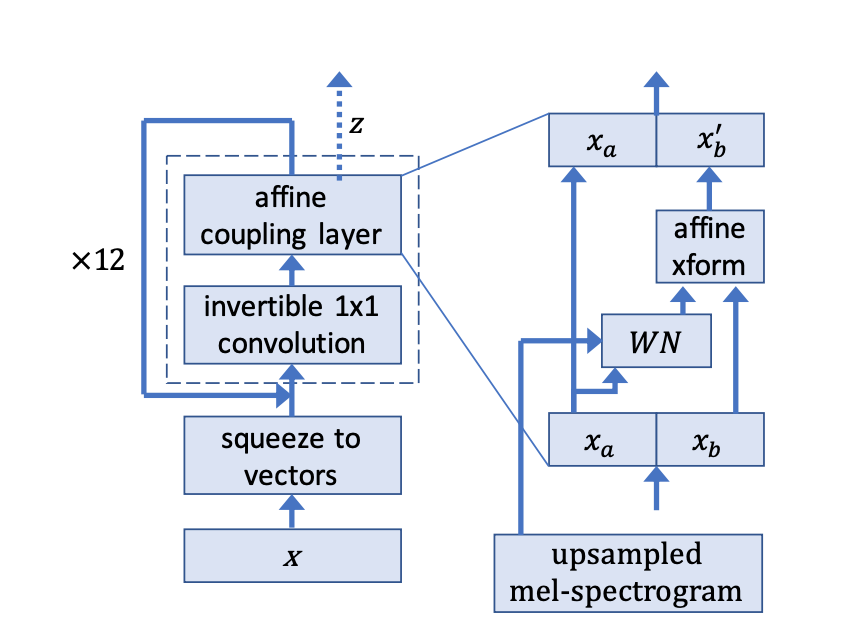
Model (WaveGlow)

WaveGlow is a flow-based model, not an autoregressive model.

waveglow

2. Acoustic Model

2.1. DNN

An alternative generative model with HMM is the DNN-HMM

DNN is a discriminative model, so it can not be directly connected with the HMM model, In the DNN-HMM hybrid model, DNN first estimates the posterior \(P(p|X)\) where \(p\) is usually a CD state, then converting this output to likelihood with prior by using

\[P(X|p) \propto \frac{P(p|X)}{P(p)}\]

Then the \(P(X|p)\) can be plugged into the generative HMM framework.

2.2. RNN

Model (location aware attention) applying 1d convolution to the previous attention when computing new attention for current timestamp.

It can be implemented with additive attention, for example,

\[a_j(q, k) = w_2^T \tanh(W[q;k] + F * a_{j-1})\]

Note

Convolution helps to move attention forward to enforce monotonic attention.

If the previous attention is \([0, 1, 2, 1, 0]\) and learned conv kernel is \([1, 0, 0]\) with pad 1 stride 1,

then output will shift by one step \([0, 0, 1, 2, 1]\)

2.3. Transformer

2.3.1. Positional Encoding

This paper compares 4 different positional encoding for transformer-based AM, convolution works best here

None
Sinusoid
Frame stacking
Convolution: VGG

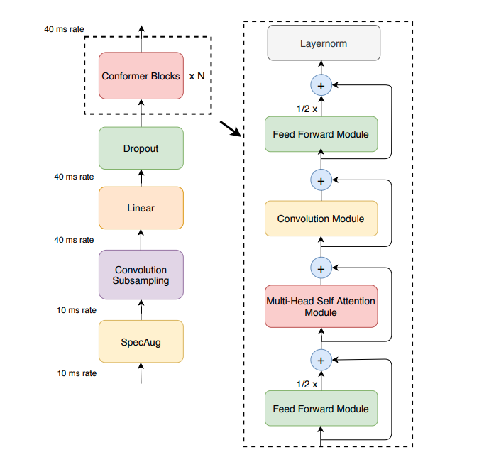
2.4. Conformer

Conformer combines self-attention and convolution

self-attention captures content-based global information
convolution captures local features effectively

number of params is roughly hidden^2*layer*23 where the constants can be broken into:

4: MLHA
8: first FFN
8: second FFN
3: inside convolution (pointwise conv=1, GLU=1, pointwise conv=1)

This is mostly 2-times larger than the transformer with same hidden size

conformer

Reference: from conformer paper

This paper has a good comparison between conformer and transformer

2.5. E2E

Instead of the traditional pipelines, we can train a deep network that directly maps speech signal to target word/word sequence

simplify the complicated the model building process
easy to build ASR systems for new tasks without expert knowledge
potential to overperform the conventional pipelines by optimizing a single objective

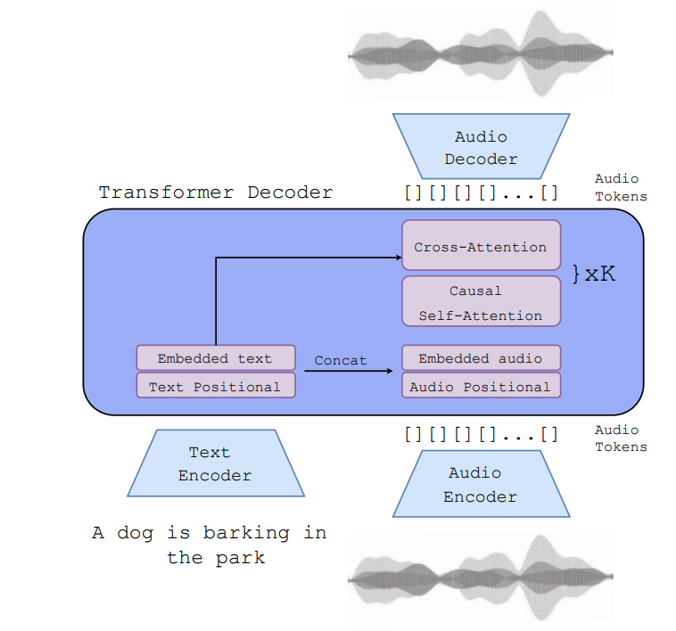
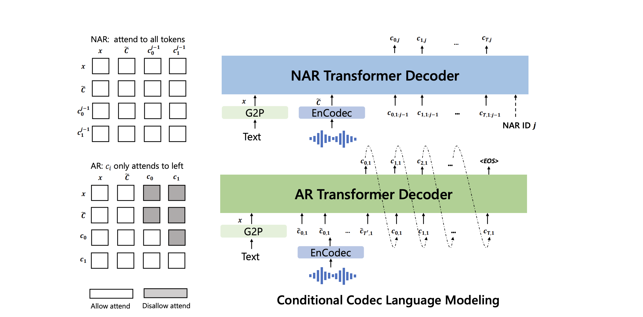
2.6. Codec Language Model

Model (AudioGen) use soundstream token and conditioned on textual description embeded with T5

audiogen

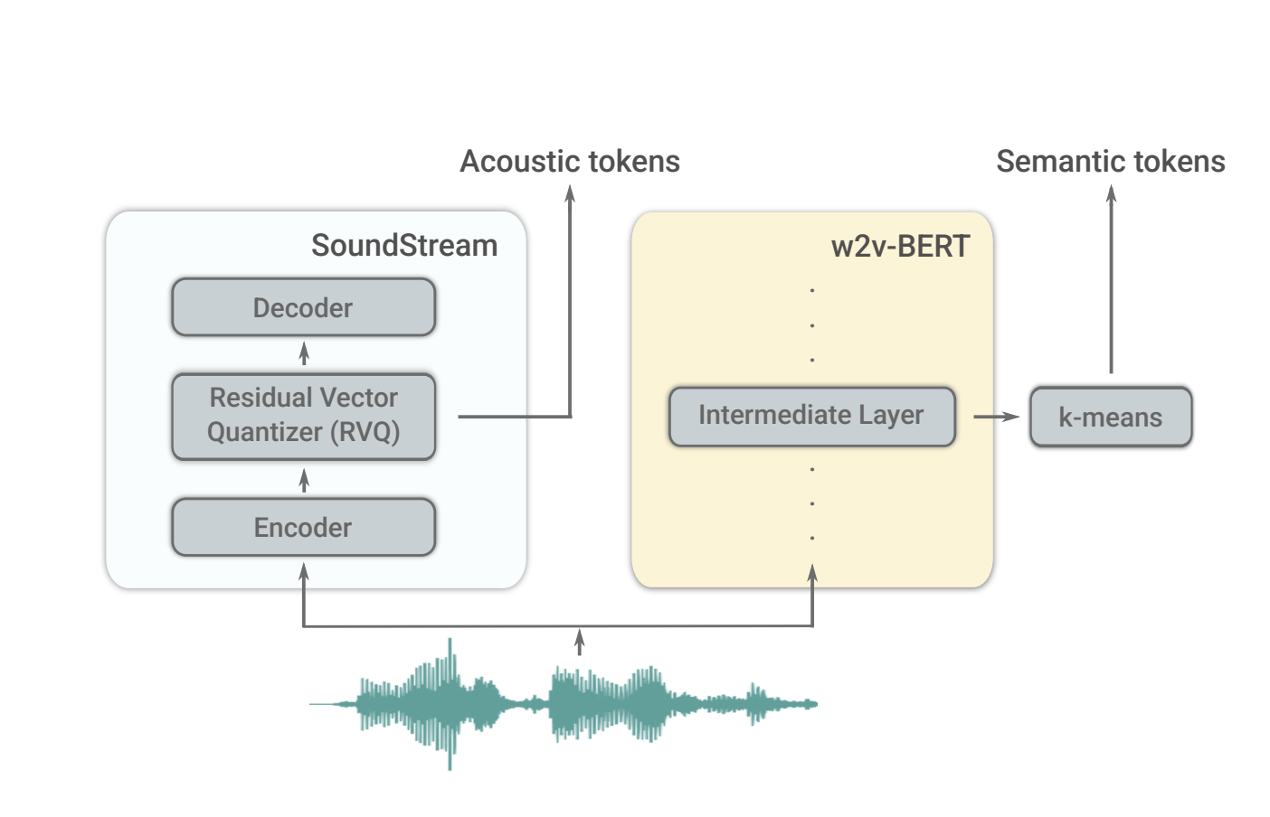
Model (AudioLM) use soundstream's token as discrete units

audiolm

Model (VALL-E) use EnCodec as discrete tokenizers

valle2

3. Alignment

We consider mapping input sequence \(X=[x_1, ..., x_U]\) to output sequence \(Y=[y_1, ..., y_T]\) where \(X,Y\) can vary in length and no alignment is provided. We are interested in the following two problems:

loss function: compute conditional probability \(-\log p(Y|X)\) efficiently and its gradient efficiently
inference: find the most likely sequence \(\hat{Y} = \text{argmax}_Y p(Y|X)\)

The following three criterions can be applied to solve this problem

3.1. ASG

ASG (Auto-Segmentation Criterion) aims at minimizing:

\[ASG(\theta, T) = - LSE_{\pi \in \text{asg}} (f_{\pi_t}(x) + g_{\pi_{t-1}, \pi(t)}(x)) + LSE_{\pi \in \text{Z}} (f_{\pi_t}(x) + g_{\pi_{t-1}, \pi(t)}(x))\]

where \(f,g\) are emission/transition scores

3.2. CTC

CTC can handle some potential problems of ASG in some cases

repeat token creates ambiguity (aabbba -> aba or abba?). An emission can map to multiple outputs
not every input frame has an label (e.g: silence)

Note for reference, see Alex Grave's thesis Chapter 7 rather than the original CTC paper. The definition of \(\beta\) in thesis is consistent with the traditional definition.

3.2.1. Training

CTC is a discrimative model, it has a conditional independence assumption for a valid alignment \(A=\{ a_1, ..., a_T\}\).

\[P(A|X) = \prod_{t=1}^T p_t(a_t | X)\]

then the objective of CTC is to marginalize all valid alignments:

\[p(Y|X) = \sum p(Y|A)p(A|X) = \sum_{A \in \mathcal{B}^{-1}(Y)} p(A|X)\]

where the sum can be done efficiently by forward computing. Note there are two different transition cases when aligned character is blank or not.

We want to minimze the negative-log-likelihood over the dataset.

\[\sum_{(X,Y) \in \mathcal{D}} -\log p(Y|X)\]

Suppose the training set is \((x,z)\) and network outputs of probability is \(y^t_k\). The objective is

\[- \frac{\partial \log p(z|x)}{\partial y^t_k} = -\frac{1}{p(z|x)}\frac{\partial p(z|x)}{\partial y_k^t}\]

Noting the \(\alpha, \beta\) has the property

\[\alpha_t(s)\beta_t(s) = \sum_{\pi \in \mathcal{B}^{-1}(z), \pi_t = z'(s)} \prod_{t=1}^T y^t_{\pi_t}\]

from which we obtain,

\[\frac{\partial \alpha_t(s)\beta_t(s)}{\partial y_k^t} = \begin{cases} \frac{\alpha_t(s)\beta_t(s)}{y_k^t} & \text{if k occurs in z'} \\ 0 \text{otherwise} \end{cases}\]

For any \(t\), we have

\[p(z|x) = \sum_{s=1}^{|z'|} \alpha_t(s)\beta_t(s)\]

We know

\[\frac{p(z|x)}{\partial y_k^t} = \frac{1}{y_k^t} \sum_{s \in lab(z, k)} \alpha_t(s)\beta_t(s)\]

3.2.2. Inference

One inference heuristic is to take the most likely output at each time stamp.

\[Y^* = \text{argmax}_A \prod_t p_t(a_t|X)\]

Beam search is also available by carefully collapsing hypothesis into equivalent set.

We can also consider language model

\[Y^* = \text{argmax}_Y P(Y|X) p(Y)^\alpha L(Y)^\beta\]

where the second term is the language model, and the last term is word insertion bonus. \(\alpha, \beta\) are hyperparameters to be tuned

Model (CTC-CRF)

Instead of the conditional independence, there are some works use CRF with CTC topology: use CRF to compute posterior, let \(\pi = (Y,A)\) be a valid alignment

\[p(Y,A | X) = p_\theta(\pi | X) = \frac{\exp{\phi_\theta (\pi, x)}}{\sum_{\pi'} \exp{\phi_\theta (\pi', x)}}\]

3.3. Transducer

Model (RNA, recurrent neural aligner)

removing the conditional independence assumption from CTC by using label of \(t-1\) to predict label \(t\)

Check this lecture video

Model (RNN-T) also extends the CTC model by removing the conditional independence assumption by adding a prediction network

\[p(Y,A|X) = \prod_{t=1}^T p_t(a_t|X, y_1, ..., y_{u-1})\]

Unlike CTC or RNA, each frame can emit multiple labels

where the current label depend on the non-blank label history \(y_1, ..., y_{u-1}\). The prediction network is believed to be classic LM, but might not be, removing the recurrecy (only depending on the last label \(y_{u-1}\)) would also yield similar result, which suggests it might only predict either an actual label or blank.

Pytorchaudio now has an implementation. Look at it here, the logits into the loss function is (batch, T_in, T_out, class), where (batch, T_in, class) is from audio encoder, and (batch, T_out, class) is from label encoder (prediction network).

Model (Transformer Transducer) propose to replace RNN with transformer with proper masking

3.4. GTC

This paper

3.5. Attention

Unlike CTC, attention model does not preserve order of inputs, but the ASR task requires the monotonic alignment, which makes the model hard to learn from scratch.