0x522 Convolution

3.1. Vanilla Convolution

Concept (receptive field) the receptive field has a closed form

\[r_0 = \sum_{l=1}^L \Bigl( (k_l-1)\prod_{i=1}^{l-1}s_i \Bigr) + 1\]

where \(r_0\) is the receptive field wrt the input layer, \(L\) is the total layer size, \(k_l, s_l\) is the kernel and stride with in layer \(l\)

Model (conv 1d) applied convolution to 1d signal

• Input: \((C_{in}, L_{in})\)
• Output: \((C_{out}, L_{out})\)
• Param: \(C_{in}C_{out}kernel\)

where \(C_{in}, C_{out}\) are input, output channels, \(L_{in}, L_{out}\) are input, output lengths

Recall the length is determined by

\[L_{out} = floor(\frac{L_{in} + 2padding - kernel}{stride} + 1)\]

When \(stride==1\), it is convenient to set \(kernel = 2padding + 1\) to maintain the same length

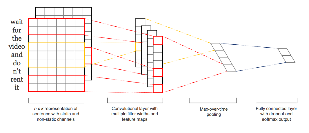
Kim's convolution network is a good illustrution of Conv 1d, where the number of words in length, and embedding size is the channel

3.2. Transposed Convolution

Transposed convolution is used to upsample dimension (as opposed to the downsampling by normal convolution). It can be used in semantic segmentation, which classifies every pixel into classes.

It is call "transposed" because it can be implemented using matrix transposition, see this chapter

3.3. Efficient Convolution

pointwise Convolution combines info across all channel in each pixel.

Model (pointwise conv, conv 1x1, network in network) It is a fully connected layer across channel dim for every pixel.

• It is to exchange information across channels for each pixel. Explained in the Network in Network
• It can be used to reduce channel size (28x28x192 -> 28x28x32)

1x1 convolution. Watch this video

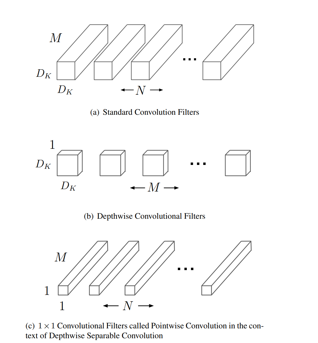
On the other side, Depthwise applies convolution within each channel.

Model (depthwise separable conv, Xception) split the standard convolution (spacial and channel convolution) into two separate conv, which helps to reduce number of params

• depthwise conv: conv per each channel (over space)
• pointwise conv: 1x1 conv (over channel)

Model (MobileNet)

Figure from the mobilenet paper

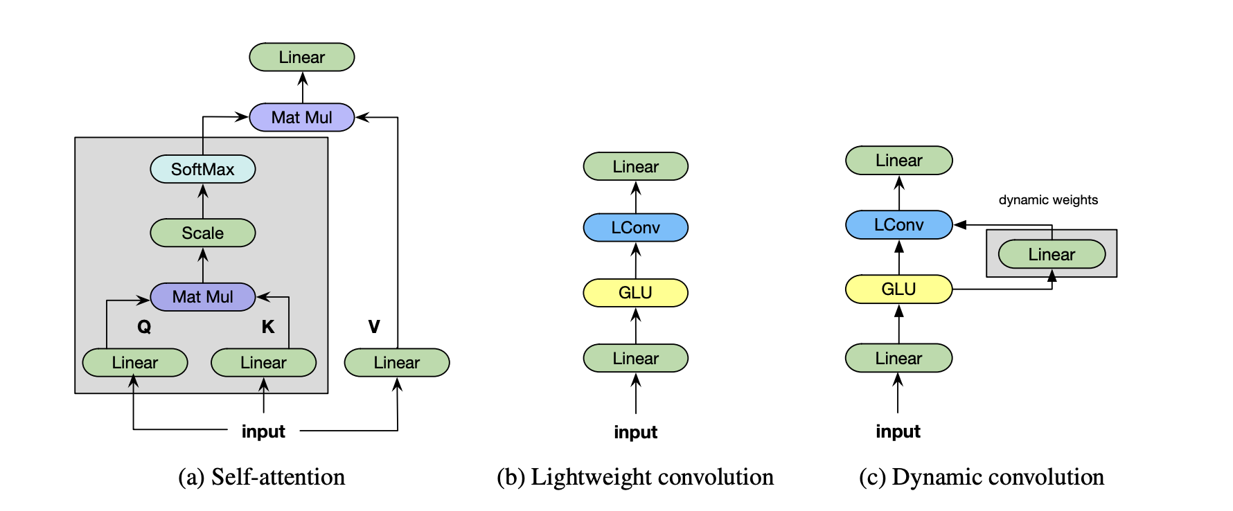
Model (lightweight convolution) proposed to replace self-attention due to simplicity and efficiency

3.4. Residual Convolution

Model (ResNeXt, Aggregated Transformation) Repeat the building blocks by adding a new dimension called cardinality \(C\) (number of the set of transformation)

\[\mathcal{F}(x) = \sum^C_i \mathcal{T}_i (x)\]

Model (DenseNet) DenseNet connects each layer to every other layer using a feed-forward connection.

Figure from densenet paper

Model (U-Net)

Model (EfficientNet)

1.1.1. R-CNN

Model (R-CNN, Region-Based CNN)

Step 1: find region proposals (maybe from some external algorithms)

Region proposal is to find a small set of boxes that are likely to cover all objects. For example, Selective Search gives 2000 regions

Step 2: wrap image regions into 224x224 and run convolutional net to predict class dsitributions and transformation of bounding box \((t_x, t_y, t_h, t_w)\)

\[b_x = p_x + p_w t_x\]

\[b_w = p_w \exp(t_w)\]

Note that weight and height are transformed in exp scale

One problem arises here is that object detctors might output many overlapping detections. The solution is to postprocess raw detections using Non-Max Suppression, it is to greedily pickup the highest scoring box and delete box whose overlap with it is high enough. This still has some open issues that it may eliminate good boxes.

Model (Fast R-CNN)

One issue with R-CNN is its very slow (running full CNN for 2000 proposals). Fast R-CNN split the full CNN into two CNN, where the first CNN (backbone network) is shared by all proposals. Most computation happens here so it is fast.

The proposed region is to take shared output from the first backbone CNN and forward through the second small CNN.

Model (Faster R-CNN)

With Fast R-CNN, most computational costs are from the region proposals, to further make it faster, Faster R-CNN uses the Region Proposal Network (RPN) to predict proposals from features

1.1.2. Modern CNN

Model (ConvNexT)