0x442 Classical Model

• 1. Speech Processing
  • 1.1. Speech Enhancement
• 2. Speech Synthesis
  • 2.1. Vocoder
  • 2.2. Concatenative TTS
  • 2.3. Parametric TTS
    • 2.3.1. Clustering
    • 2.3.2. Modeling
      • 2.3.2.1. Duration Model
      • 2.3.2.2. Observation Model
      • 2.3.2.3. DNN Model
• 3. Speech Recognition
  • 3.1. Acoustic Model
    • 3.1.1. HMM
      • 3.1.1.1. Triphone HMM
    • 3.1.2. GMM
    • 3.1.3. Speaker Adaptation
  • 3.2. Language Model
    • 3.2.1. Search Algorithm
      • 3.2.1.1. Viterbi search
      • 3.2.1.2. Forward search
    • 3.2.2. Discriminative Training
      • 3.2.2.1. MMI
      • 3.2.2.2. MBR
      • 3.2.2.3. Lattice-free MMI
    • 3.2.3. Automata
      • 3.2.3.1. FST
      • 3.2.3.2. Differentiable WFST
    • 3.2.4. Rescoring
• 4. Reference

1. Speech Processing

1.1. Speech Enhancement

Evaluation (PESQ, Perceptual evaluation of speech quality) evaluation metric

2. Speech Synthesis

2.1. Vocoder

Vocoder takes the acoustic features (mel spectrogram) into a time-domain audio waveform

Model (Griffin Lim): reconstructing phase

2.2. Concatenative TTS

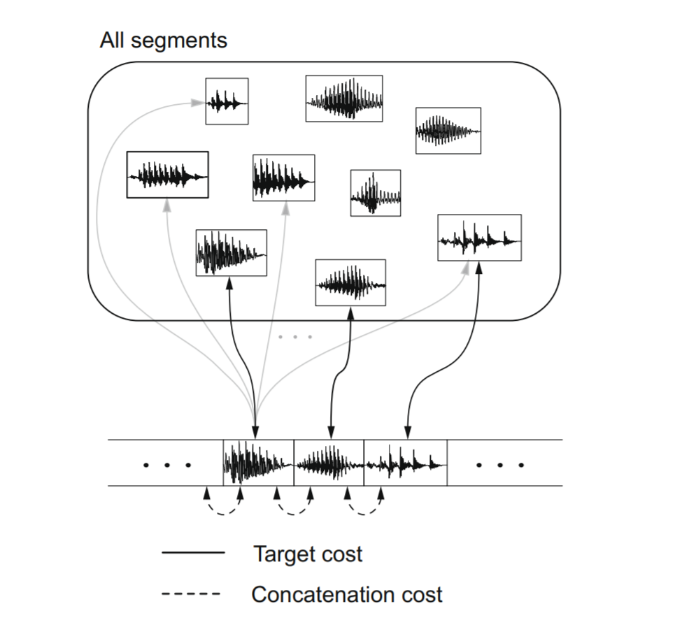
The basic unit-selection premise is that we can synthesize new natural-sounding utterances by selecting appropriate sub-word units from a database of natural speech. The subword units might be frame, HMM state, half-phone, diphone, etc.

There are two costs to consider when concatenating units.

Target cost is about how well a candidate unit from the database matches the required units.

\[C_{target}(t_i, u_i) = \sum_j w_j C^{target}_j(t_i, u_i)\]

where \(u_i\) is a candidate unit and \(t_i\) is a required unit and \(j\) sums over the features (e.g: phonetic, prosodic contexts.)

The other cost is Concatenative cost, which defines how well two selected units combines

\[C_{concat}(u_{i-1}, u_i) = \sum_k w_k C^{concat}_k(u_{i-1}, u_i)\]

where \(k\) sums over the features (e.g: spectral and acoustic features)

The goal is to find a string of units \(u=\{ u_1, ..., u_n \}\) from the database that minimizes the overall costs

\[\hat{u} = \text{argmin}_u \sum_i C_{target}(t_i, u_i) + C_{concat}(u_{i-1}, u_i)\]

2.3. Parametric TTS

Statistical parametric speech synthesis might be most simply described as generating the average of some sets of similarly sounding speech segments.

In a typical parametric system, the steps are training phase and synthesis phase

In the training phase, we first extract parametric representations of speech (e.g: spectral, excitation) and model them using a generative model (e.g.: HMM), estimated with MLE

\[\hat{\lambda} = \text{argmax}(P(O | W, \lambda))\]

where \(\lambda\) is the parameter, \(O\) is the training set and \(W\) is the word sequence of \(O\)

In the synthesis phase, we want to generate a speech, we use the estimated parameter \(\hat{\lambda}\) and target words \(w\).

\[\hat{o} = \text{argmax}(P(o | w, \hat{\lambda}))\]

The flow of HTS is as follows:

2.3.1. Clustering

Typically, we want to create a model to map the a set of linguistic features to the acoustic feature. However, there are many unseen contexts (linguistic feature) in the corpus. We need to make generalization from the limited number of observed samples to unlimited number of unseen contexts.

For example, we can use the clustering approach to tie parameters to achieve generalization

In CLUSTERGEN, CART trees are built in the normal way with wagon to find questions that split the data to minimize impurity. The impurity is calculated as

\[N\sum_i \sigma_i\]

Where N is the number of samples in the cluster and σi is the standard deviation for MFCC feature i over all samples in the cluster. The factor N helps keep clusters large near the top of the tree thus giving more generalization over the unseen data.

2.3.2. Modeling

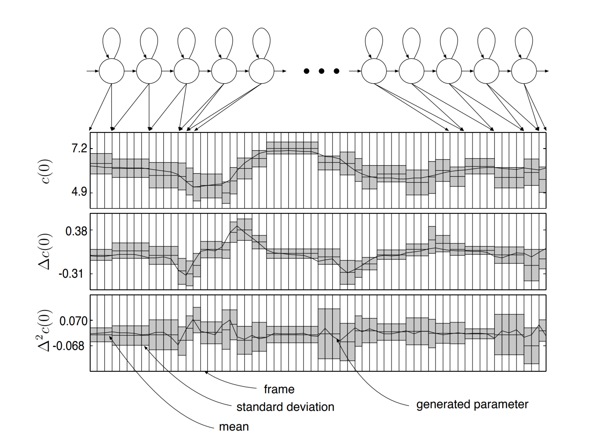
2.3.2.1. Duration Model

Model (duration) the durations (i.e. the number of frames of parameters to be generated by each state of the model) are determined in advance – they are simply the means of the explicit state duration distributions.

2.3.2.2. Observation Model

The naive approach to generate the most likely observation from each state is to take the mean of Gaussian, which would generate piecewise constant trajectories, which is not natural, so we have the MLPG algorithm

Model (maximum likelihood parameter generation, MLPG) Model the delta and delta-delta as well, illustrated in the following

2.3.2.3. DNN Model

Instead of the Gaussian model, we can use a DNN for observation instead

This tutorial is very helpful

3. Speech Recognition

Speech recognition is a task modeling relation between speech input \(O\) and linguistic (text output) \(W\), the task is to find \(W\) such that

\[\text{argmax}_W P(W|O)\]

The formulation can be decomposed into the followings:

\[P(W|O) = \sum_L P(W,L | O) = \sum_L P(O | L, W) P(L,W) = \sum_L P(O|L)P(L|W)P(L)\]

where

• \(P(O|L)\) is the acoustic model
• \(P(L|W)\) is the pronounciation model
• \(P(W)\) is the language model

3.1. Acoustic Model

3.1.1. HMM

For the note of HMM model itself, see the structure learning note

3.1.1.1. Triphone HMM

How to represent each triphone HMM state as a single Gaussian:

• bottom up: computationally heavy, missing triphones
• top down: use phonetic information

3.1.2. GMM

GMM-HMM is one of the traditional generative models.

Delta feature relax the conditional indepedence assumption in HMM/GMM.

3.1.3. Speaker Adaptation

MAP

MLLR

Comparison:

• low resource: MLLR > MAP > ML
• middle resource: MAP > MLLR == ML
• high resource: MAP == ML > MLLR

3.2. Language Model

3.2.1. Search Algorithm

3.2.1.1. Viterbi search

Search a single path with max score

3.2.1.2. Forward search

Compute logsumexp of all possible paths

3.2.2. Discriminative Training

3.2.2.1. MMI

This slide

3.2.2.2. MBR

3.2.2.3. Lattice-free MMI

3.2.3. Automata

Much of current ASR models usch as HMM, tree lexicon, n-gram language model can be represented by WFST. Recall they can encode regular relations. It maps an input from regular language \(X\) to another regular language \(Y\).

Even richer model such as context-free grammar in spoken-dialog applications, they are usually restricted to regular subsets due to efficiency reasons.

3.2.3.1. FST

The most important and expensive operation is composition, where the complexity is \(O(V_1V_2D_1D_2)\) where \(V_1, V_2\) are number of nodes, \(D_1,D_2\) are the max out-degrees. Potential solution are on-the-fly composition (dynamic composition)

3.2.3.2. Differentiable WFST

Most of the materials here are from Awni's Interspeech tutorial and CMU 11751 lecture.

why differentiable with Automata?

• combine training and decoding
• separate data (graph) and code (operations)

Differentiation is defined wrt the graph (actually, weights in the graph).

Graph has an analogy to tensor. Composition of graphs (e.g: concatenation) is like composing tensors (e.g: multiplication). Here are some examples:

operation type	Tensor	Graph
unary	power, negation	closure
binary	multiplication	intersection, compose
reduction	sum, max, prod	shortest distance
n-ary	addtion, subtraction	concatenation, union

3.2.4. Rescoring

This paper introduces N-Best List rescoring

4. Reference

[1] festvox book

[2] Zen, Heiga, Keiichi Tokuda, and Alan W. Black. "Statistical parametric speech synthesis." speech communication 51.11 (2009): 1039-1064.

[3] Taylor, Paul. Text-to-speech synthesis. Cambridge university press, 2009.

[4] King, Simon. "A beginners’ guide to statistical parametric speech synthesis." The Centre for Speech Technology Research, University of Edinburgh, UK (2010).

[3] There is a chapter in Festvox book describing how to develop TTS prompts