0x404 Nonparametric Models
- 1. Frequentist Estimation
- 2. Bayesian Estimation
- 3. Minmax Risk Lower Bound
- 4. Asymptotics
- 5. Reference
An important limitation of parametric model is that the chosen density might be a poor model of the true distribution (e.g: Gaussian model is a poor model of the multimodal distribution). The nonparametric model make few assumptions about the form of the distribution.
In nonparametric model, we assume the distribution \(p\) belongs to some "massive" class \(\mathcal{P}\) of densities. For example, \(\mathcal{P}\) can be the set of all continuous probability density or Lipschitz continuous probability density.
1. Frequentist Estimation
To estimate the probability density at a particular location, we should consider the data points that lie within some local neighbourhood of that point. Let us consider some small region \(\mathcal{R}\) containing \(x\), the probability of this region is given by
Suppose we have \(N\) data points, the number of points falling inside the region \(K\) is rouhgly \(K \sim NP\). Assume the region \(\mathcal{R}\) has constant probability over the region volume \(V\), then
we have the density estimate
where \(K,V\) are interdependent on each other.
1.1. Nearest Neighbor
1.1.1. Density Estimation
NN approach fixes \(K\) to find an appropriate \(V\). In the Nearest-Neighbor density estimation, we allow the radius of sphere from \(x\) to grow until it contains precisely \(K\) data point. then we apply the estimation
1.1.2. Classification
The density estimation can be extended to the classification problem. we draw a sphere centred on \(x\) containing \(K\) points: \(N_k\) from class \(C_k\). then density for each class is
Suppose the unconditional density is \(p(x) =K/NV\) and priors are \(p(C_k) = N_k/N\), we obtain the posterior as
Maximizing the probability of misclassification is to identify the largest number \(K_k\)
1.1.3. Search
In the low-dimension, KD-tree is effective, but in high-dimensional, nearest neighbor search is expensive due to the curse of dimensionality.
paper (jegou2010product) Product quantization for nearest neighbor search
- quantization step: split the vector \(x \in R^D\) into \(m\) distinct subvectors \(u_i(x) \in R^{D^*}\) where \(mD^* = D\), apply subquantizer \(q_i\) (k-means) to each subvector.
- seach step: quantize both key and query or quantize only key. All key's subvector distance should be precomputed. In the first case, the key-query comparison is reduced to \(m\) addition.
- nonexhaustive search: Follow Video-Google paper, use two quantizers applied to keys (coarse quantizer and residue quantizer), use coarse quantizer to lookup a inverted index, then go through the list using the residue.
1.2. Kernel Density Estimation
Kernel Density Estimation is to fix \(V\) and determine \(K\) from data. Let the empirical distribution function be
For sufficiently small \(h\), we can write the approximation with $p(x) = (F(x+h) - F(x-h))/2h, which gives rise to the Rosenblatt estimator
where \(K_0 = \frac{1}{2} I(-1 \leq u \leq 1)\).
Estimator (Kernel Density Estimator, Parzen-Rosenblatt) A simple generation is given by
where \(K\) is called kernel and should be normalized to 1 \(\int K(u) du = 1\), \(h\) is called bandwidth
1.2.1. MSE Analysis
The MSE at an arbitrary fixed point \(x_0\) is
which, as usual, can be decomposed to bias and variance
where bias is
and variance is
Proposition (variance upper bound) Suppose the density \(p(x)\) satisfies \(p(x) < p_{max} < \infty\) for all \(x \in R\) and \(\int K^2(x) dx < \infty\), then
where \(C_1 = p_{max}\int K^2(x) dx\)
Definition (Holder class) Let \(T\) be an interval in \(R\) and \(\beta\), \(L\) be positive. The Holder class \(\Sigma(\beta, L)\) on \(T\) is defined as the set \(l = \lfloor \beta \rfloor\)-times differentiable function such that
Definition (order of kernel) We say kernel \(K\) is a kernel of order \(l\) if the function \(u^j K(u)\) is integrable for \(j = 0, 1, ..., l\) and
Proposition (bias upper bound) Assume \(p \in \Sigma(\beta, L)\) and \(K\) be a kernel of order \(l = \lfloor \beta \rfloor\) satisfying
Then for all \(x_0, h > 0, n\geq 1\) we have
where \(C_2 = \frac{L}{l!} \int |u|^{\beta} |K(u)| du\)
Lemma (risk upper bound) By the previous analysis, we know
Notice when \(h\) is increasing, the bias increases but variance decreases. Setting up the correct \(h\) is important.
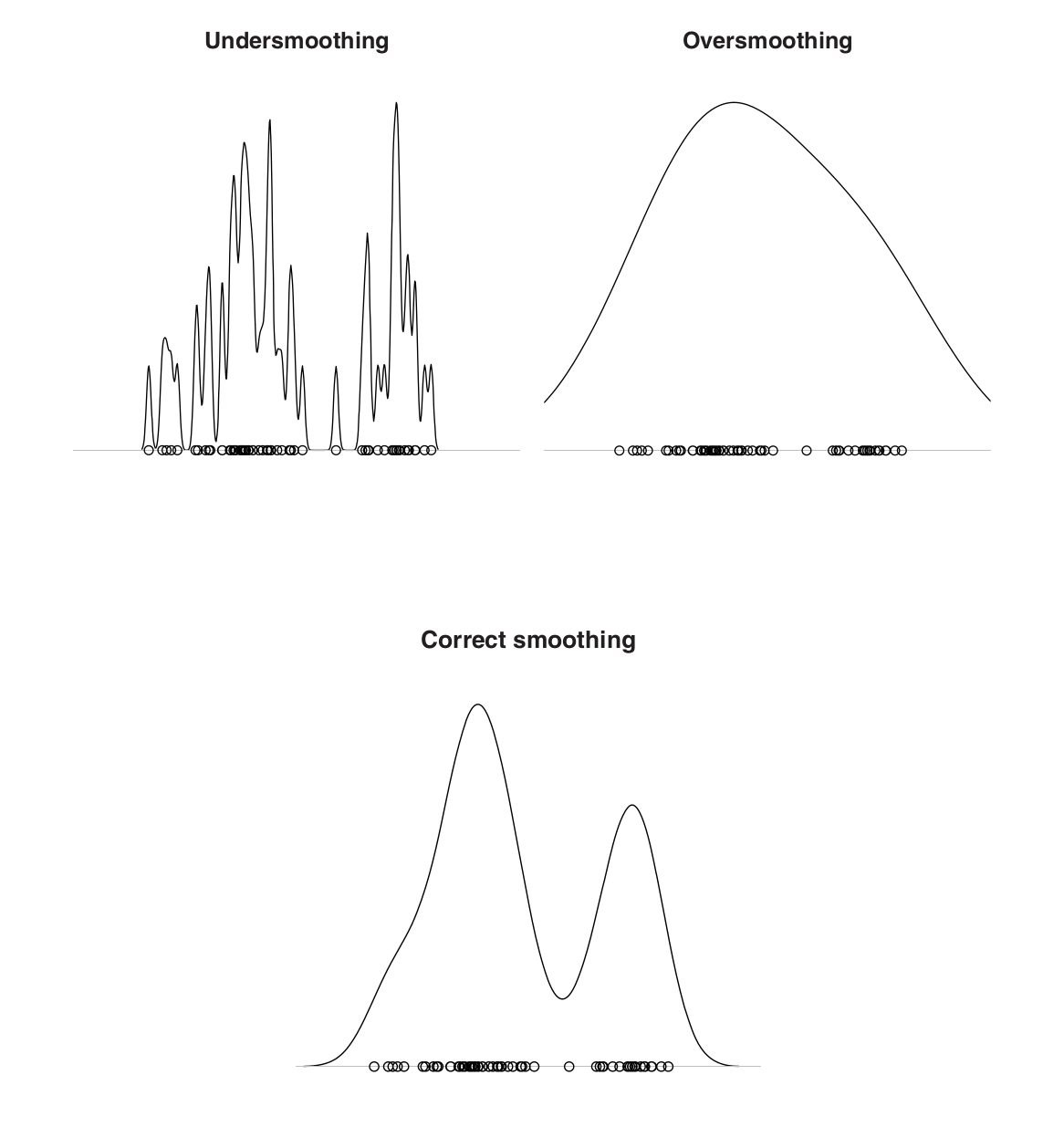
Optimizing the previous objective, we obtain
1.3. Kernel Regression
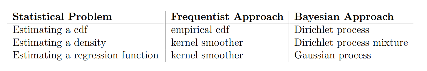
2. Bayesian Estimation
Larry's PDF is very good
2.1. Gaussian Process
Recall a Gaussian distribution is specified by a mean vector \(\mu\) and covariance matrix \(\Sigma\)
Gaussian Process is a generalization of multivariate Gaussian distribution to infinitely many variables.
Definition (Gaussian Process) GP is a collection of random variables, any finite number of which have consistent Gaussian distributions. The general form is fully specified by a mean function \(\mu(x)\) and a covariance function \(K(x, x')\).
2.1.1. GP Regression
In the GP regression viewpoint, instead of modeling the prior over parameters \(w \sim \mathcal{N}(0, \alpha^{-1} I)\), we define the prior probability over \(f(x)\) directly
In practice, we observe \(N\) data points, which have the distribution
where \(K_n\) is the Gram matrix
Further considering the observed taret values is modeled by
The marginal distribution becomes
where the covariance matrix is
Further considering the new data point \(t_{N+1}\), the joint distribution is
where \(C_{N+1}\) is defined as
Applying the conditional rules \(P(t_{N+1} | t_{1:N})\), we know
The central computational operation is the inversion of \(C_N\) matrix \(N \times N\), usually \(O(N^3)\)
Some useful links:
2.2. Dirichlet Process
Dirichlet Process is a generalization of Dirichlet distribution which model the prior of infinite mixture models.
It is specified by
-
base distribution \(H\): expected value of the process (mean of drawed distribution)
-
concentration positive parameter \(\alpha\): a smaller \(\alpha\) indicates a higher concentration
The process is modeled by
It can be interpreted sequentially such that
It can be used, for example, to model the clustring without predefining the \(k\) cluster size
3. Minmax Risk Lower Bound
4. Asymptotics
5. Reference
[1] Tsybakov, Alexandre B. "Introduction to Nonparametric Estimation." Springer series in statistics (2009): I-XII.