0x501 Optimization
- 1. Optimization
- 2. Regularization
- 3. Reference
1. Optimization
This note only covers deep-learning related optimization, this is the note for more general continuous convex optimization discussion
1.1. Online Learning
Unlike PAC learning framework:
- The online learning framework mixes the training and testing instead of separating them
- does not make any distributional assumption (in PAC framework, the data distribution is considered fixed over time)
The performance of online learning algorithms is measured using a mistake model and the notion of regret, which are based on a worst-case or adversarial assumption
The objective is to minimize the cumulative loss \(\sum_{t=1}^T L(\hat{y}_t, y_t)\) over \(T\) round
Definition (regret) regret measure the difference between current model and the best model (inf over i in the following formula)
1.2. Forward Gradient
backprop is unfortunately
- considered as “biologically implausible”
- incompatible with a massive level of model parallelism
Model (weight perturbation, directional gradient descent) update the parameters of the representation by using the directional derivative along a candidate direction
Another relevant work is this one
Model (activity perturbation) yields lower-variance gradient estimates than weight perturbation and provide a continuous-time rate-based interpretation of our algorithm
1.3. Backward Gradient
Most of the popular optimizers are roughly variants of the following framework
General Framework:
- compute grad \(g_t = \nabla f(w_t)\)
- compute 1st and 2nd moments \(m_t, V_t\) based on previous grads \(g_1, ..., g_t\)
- compute updating grad \(g_t = m_t/\sqrt{V_t}\) and grad descent
Model (SGD) no moments
1.3.1. Momentum (1st moments)
Model (SGD with momentum) update momentum as follows
Model (Nesterov Accelerated Gradient, NAG) move first and then compute grad and make a correction, check Hinton's slide
1.3.2. Adaptive learning (2nd moments, magnitude)
Model (adagrad) works in sparse dataset. using magnitude to change the learning rate: \(\alpha \to \alpha / \sqrt{V_t}\)
Model (RMSProp) using moving average for magnitude
Model (adam) RMSProp + Momentum with the unbiased adjustion
Model (nadam) adam + nesterov
Model (adamw) adam + weight decay
1.3.3. Batching
Analysis (large batch is bad at generalization) This work claims large-batch methods tend to converge to sharp minimizers, which has poorer generalization.
Goyal et al. 2017 shows the learning rate should be scaled linearly with the global batch size together with a warmup stage. There are also discussion that learning rate should be sqrt of the batch size to keep the variance
This paper suggests increasing the batch size instead of decreasing learning rate
1.4. Hessian Methods
Even hessian is not explicitly computed, information of Hessian such as trace, spectrum can be extracted using numerical algebra or its randomized version.
These information is helpful, for example, to analyze model's generalization
1.4.1. Matrix-free Methods
1.4.1.1. Trace
Suppose we can query \(Ax\) without knowing \(A \in \mathbb{R}^{n \times n}\) explicitly, we want to approximate \(tr(A)\)
One simple idea is to
which requires \(n\) queries and might not be efficient
Model (Hutchinson's method)
draw \(x_1, ..., x_m\) from random \(\{ -1, 1 \}\) (i.e., Rademacher distribution), then the estimator of \(tr(A)\) is
The validity of this estimator can be derived using Hanson-Wright inequality, which states the concentration result for quadratic forms in sub-Gaussian random variables
1.4.1.2. Spectrum
Model (Stochastic Lanczos Quadrature)
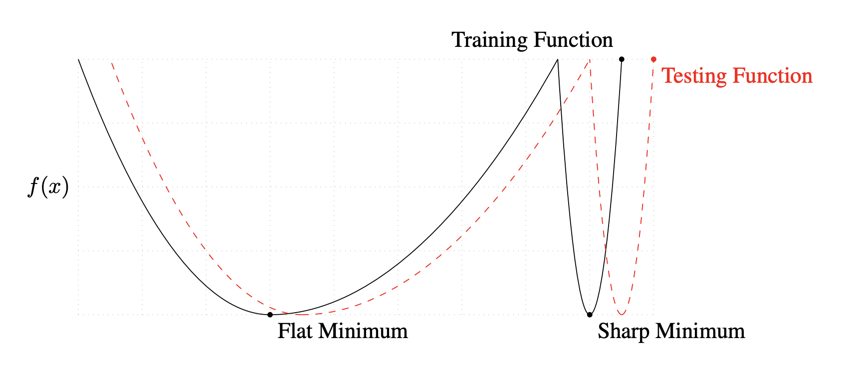
1.4.2. Loss Topology
landscape, flatness, sharpness
Model (sharpness, Keskar) largest eigenvalue of loss to characterize the sharpness, large batch size tends to generalize less well
1.5. Bayesian Optimization
Bayesian Optimization can be used to find hyperparameters. It builds a probabilistic proxy model for the objective using outcomes of past experiments as training data.
1.6. Others
Model (meta learning, MAML) optimize parameter to minimize 1-step further loss over a new task
where \(\theta'_i\) is one step updated parameter
2. Regularization
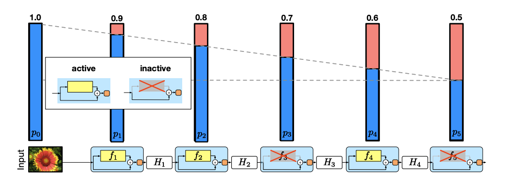
2.1. Dropout
Model (stochastic depth) randomly drop at the layer-level with the dropping probability linearly changes wrt depth
2.2. Normalization
Batch Norm normalize over the batch dim
where \(\gamma, \beta\) are learnable parameters
Benefits of using batch norm are
- reduce covariate shift as claimed by the original paper
- enable larger learning rate without exploision, shown by this work
- makes the optimization landscape significantly smoother: improvement in the Lipschitzness of the loss function as shown by this work
Batch norm is not appropriate when
- used in RNN where stats across timestamps vary
- batch size is small, try using batch renormalization instead (with the cost of more hyperparameter)
- reduces robustness to small adversarial input perturbations as shown by this work
WeightNorm normalize inputs with L2 norm of weights instead of inputs (i.e. \(\mathbf{w} = g \mathbf{v}/|\mathbf{v}|\)) but is less stable so not widely used in practice.
LayerNorm normalize over the layer dim by leveraing re-centering and re-scaling invariance. RMSNorm argues re-centering invariance is not important and it only aplies re-scaling.
Group Norm divides the channels into groups and computes within each group the mean and variance for normalization
2.3. Data Smoothing
Model (label smoothing)
Model (confidence penalty) penalizing low-entropy
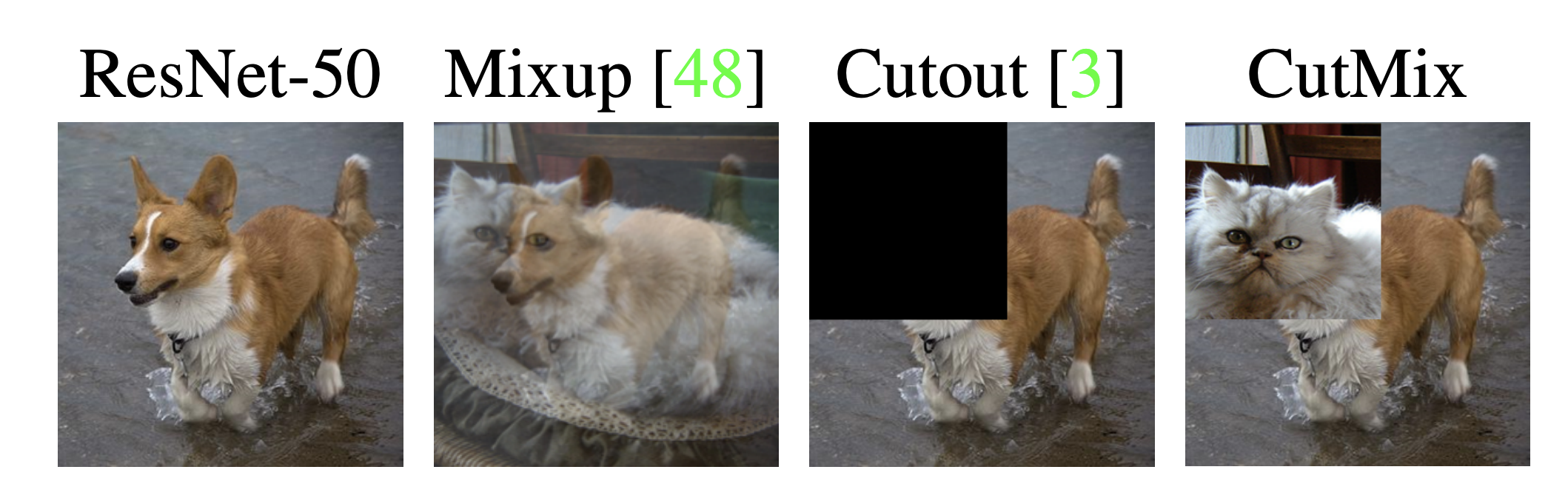
Model (mixup) Instead of minimizing empirical risk, mixup minimizes Vicinal Risk (introduced in this paper), where virtual examples are drawn from vicinity distribution
where \((\tilde x, \tilde y)\) are in the vicinity of the training feature-target pair \((x_i, y_i)\).
In this work, \((\tilde x, \tilde y)\) was implemented as a linear combination of two data points \((x_1,y_1)\) and \((x_2, y_2)\)
where \(\lambda\) is sampled from beta distribution
Model (cutmix) see the following diagram