0x500 Theory
1. Automatic Differentiation
Check this video
To follow the video, we are using numerator notation here:
Let \(f: \mathbb{R}^n \to \mathbb{R} = D \cdot C \cdot B \cdot A = D(C(B(A(\mathbf{x}))))\)
where \(\mathbf{x}\) can be thought as weights and the scalar \(y\) is the target label
The Jacobian \(f'(\mathbf{x}) \in R^{1 \times n}\) is a multiplication of a few other Jacobian matrices:
There are many ways to order the multiplication, typically,
1.1. Forward-Mode
This is push-forward computing, it computes \(\frac{\partial \mathbf{b}}{\partial \mathbf{x}}\) everytime from right side:
and
It is convenient to be combine with Jacobian-vector product (JVP)
1.1.1. JVP
Jax implement forward-mode with JVP, it is a way to get a Python function for evaluating
Its interface is jvp :: (a -> b) -> a -> T a -> (b, T b) where T a is a tangent vector
For example, if \(f: \mathbb{R}^n \to \mathbb{R}^m\), then \(\partial f(x): \mathbb{R}^n \to \mathbb{R}^m\), \((x,v): (\mathbb{R}^n, \mathbb{R}^n)\) and \((f(x), \partial f(x) v): (\mathbb{R}^m, \mathbb{R}^m)\)
jvp algebra with dual number we can represents algebra over jvp using dual number, it augmenting real \(a\) to a tuple \(a + b\epsilon\) where \(a\) is primal, \(b\) is tangent and \(\epsilon^2 = 0\) which gives the primitives such as
See this doc how to implement jvp for a new Jax primitive
# f(x) = log(x) => f'(x) v = v/x

def log_jvp(x, v):
    return lax.div(v,x)
1.1.2. Jacobian
To obtain a full Jacobian, we can repeat JVP for every column
In Jax, we compose jvp, vjp with vmap into jmp and mjp, then implement jacfwd, jacrev
1.2. Reverse-Mode
This is pull-back computing, it computes \(\frac{\partial y}{\partial b}\) everytime from left side:
and
Similarly, it is convenient to be combined with vector-Jacobian product (VJP)
To build full Jacobian we build one row at a time:
In neural network, where Jacobian is a 1 row vector, we prefer the reverse accumulation
Comparison of forward vs reverse:
- reverse-mode requires memory cost, which scales like depth of program
- forward-mode requires \(n\) calls
1.2.1. Transpose
in jax, reverse-mode is implemented with forward-mode and transpose. paper
in addition to jvp, transponse has to be implemented
2. Theory
Recall from the PAC framework, assume we have a training dataset \(D_n = \{(x_i, y_i)\}^n_{i=1}\) drawn from the joint distribution \(X,Y \sim \mathcal{D}\)
Definition (empirical risk) The empirical risk is defined wrt to a neural network \(h \in \mathcal{H}\)
By trying to minimize the empirical risk, we trained an network \(\hat{\theta}_{\text{ERM}}\) such that
Definition (true risk, generalization error) The true risk is defined wrt to any estimator \(\hat{\theta}\) and the underlying distribution
By considering the Bayes error \(R^*\), which is the achievable lowest error by any measurable function: \(X \to Y\)
Definition (risk decomposition) The risk can be decomposed into
where \(h^* = \inf_{h \in \mathcal{H}} R(h)\)
- approximation error: first term \(|R(h^*) - R^*|\) shows how good is the empirical risk minimization of \(\mathcal{H}\) can fit to the training set \(D\), usually inaccessible
- estimation error second term \(|R(h) - R(h^*)|\) measures the quality of the hypothesis vs the best one in the hypothesis set \(\mathcal{H}\)
Under the ERM framework: \(h = \hat{h}_{\text{ERM}}\), the estimation error can be bound by complexity error: \(\sup_{h \in \mathcal{H}} | R(h) - \hat{R}(h)|\)
The complexity error can be bound by Rademacher complexity, which is further bound by VC dimension, covering number, Dudley integral etc
2.1. Approximation Theory
This subsection is related to the approximation error:
Theorem (universal approximation) MLP are universal approximators. This paper is one of the paper proving this statement
boolean function
An MLP is a universal boolean function
It can represent a given function only if it is sufficiently wide and sufficiently deep. Sometimes the depth can be traded off for exponential growth of width
Optimal width and depth depends on the number of variables and the complexity of the Boolean function
continuous function
Neural network with relu activation can approximate a random continous function. The approximation is achieved by connecting many piecewise linear functions. Intuitively, 1 neuron can provide at least 1 linear piecewise, which might be increased significantly in the deep layer.
In the case of 1 layer shallow network to approxmiate a random L-Lipshitz function, we can break the domain into \(O(L/\epsilon)\) piecewise linear function where \(\epsilon\) is the maximum tolerance.
In the case of deep neural network, we can build following blocks to approximate any random function
- \(y=x^2\) can be efficiently approximated by deep networks
- \(y=x_1 x_2\) can be built from previous block
- \(y=x^n\) can be built from the second block
- A random polynomial can be built from the 3rd block
- Any random continous function can be approximated by the Weierstrass approximation theorem
2.2. Generalization Theory
This subsection is related to the estimation error or its bound (complexity error)
One traditional bound of this is by the Dudley's integral
In neural network, the rate wrt to the number of parameter \(W\) and number of layer \(L\) is
This bound shows larger parameter and layer leads to larger estimation error, which contradicts with the current trend of large models with large parameters.
A few modern directions to interpret the neural network's generalization ability are:
2.2.1. Implicit Regularization
Neural networks can be regularized implicitly in many forms,
For example, by the learning algorithms:
Model (SGD for linear model) For linear models, SGD always converges to a solution with small norm.
Model (SGD for matrix factorization) gradient descent on factorization converges to the minimum nuclear norm solution.
2.2.2. PAC Bayes
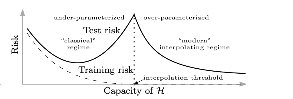
2.2.3. Double Descent
Model (double descent) overparameterizing over a threshold makes the model smoother (low norm)
3. Representation Learning
Check this chapter of deep learning book
3.1. Discrete Representation
Model (cross entropy, NLL + softmax) Let \(t\) denote the correct label, \(z\) denote logits, then \(y = softmax(z)\), cross entropy optimizes the negative loglikelihood
Taking the derivative leads to a simplified form:
However, cross-entropy have several generalization shortcomings such as
- lack of robustness to noisy labels
- poor margins.
3.2. Continuous Representation
3.2.1. Classical Metric Learning
Check the first part of this slide
Metric learning learns a distance function \(D(x, x'; \theta)\) using datasets such as \(\mathcal{S} = \{ (x_i, x_j): x_i, x_j\text{ are similar} \}, \mathcal{D} = \{ (x_i, x_j): x_i, x_j\text{ are not similar} \}, \mathcal{R} = \{ (x_i, x_j, x_k): x_i\text{ is more similar to } x_j\text{ than to } x_k \}\)
The goal is to solve the optimization problem with some loss function \(l\) and regularization \(reg\)
Distance (Mahalanobis) A classical linear metric learning is to learn a matrix \(L\)
or equivalently using a PSD matrix \(M\)
Model (linear Clustering, Xing et al 2002) The following formulation
Model (large margin nearest neighbor, Weinberg et al 2009) The following SDP
where the slack variable \(\xi_{ijl} \geq 0\) is used to measure the amount by which the large margin inequality
3.2.2. Contrastive Learning
Contrastive learning learns continuous representations \(f(x)\) of input \(x\) from both positive labels and negative labels.
See this blog
Model (contrastive loss) minimize the metric \(\| f_\theta(x_1) - f_\theta(x_2)\|\) when they are from the same class, otherwise maximize.
The most simple way is the linear model \(f_\theta(x) = Lx\) with L2 distance
Model (triplet loss)
Model (NCE loss, noise contrastive estimation) see the bayesian notes
Model (Info NCE, CPC) We want to find a way to preserve mutual information between future representation \(z_t\) and current context representation \(c_t\)
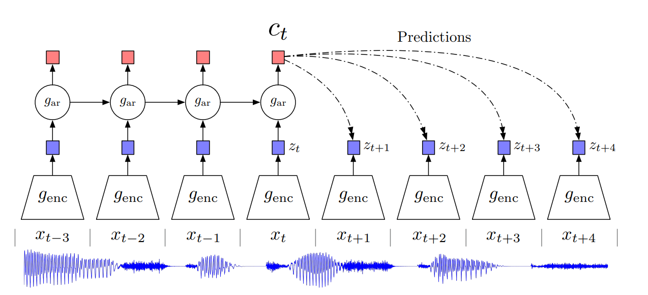
It has three representations:
- raw input \(x_t\)
- local latent feature \(z_t = g_{enc}(x_t)\)
- context feature \(c_t = g_{ar}(z_{<t})\)
CPC tries to learn a representation future \(x\) and context \(c\) such that preserves the mutual information between them
where the density ratio is modeled by
It is then optimized by the NCE loss
Optimizing this loss is equivalent to optimizing categorical cross entropy whose probability is \(P(d=i | X, c_t)\), and optimizing this loss will result in \(f_k(x_{t+k}, c_t)\) estimating the density ratio
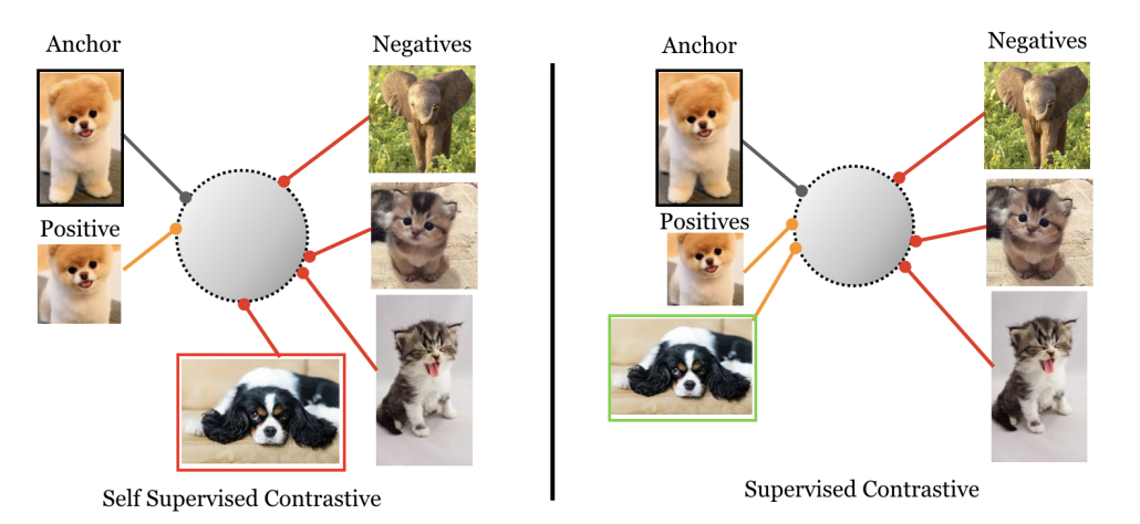
Model (supervised contrastive loss) more robust than cross-entropy by pushing embeddings from same class together
3.3. Set Representation
Model (set-input problems) input that are permutation invariant.
A function \(f(x)\) is permutation variant over countable domain can be decomposed into
This is both sufficient and necessary. Proof is simple and available at its appendix
\(\phi, \rho\) can be model with neural network, and can be regarded as encoder, decoder in this work
4. Architecture
4.1. Implicit Models
check the tutorial here
4.1.1. Neural ODE
4.1.2. Deep Equilibirum Model
4.2. Adaptation
check this talk
Let a neural network \(f_\theta: \mathcal{X} \to \mathcal{Y}\) be decomposed into a composition of functions \(f_{\theta_1} \odot f_{\theta_{2}} \dot ... \odot f_{\theta_{l}}\). each has parameters \(\theta_i\)
A module with parameters \(\phi\) can modify the \(i\)-th subfunction as follows:
- Parameter composition: \(f'_i(x) = f_{\theta_i \oplus \phi}(x)\)
- Input composition: \(f'_i(x) = f_{\theta_i}([x, \phi])\)
- Function composition: \(f'_i(x) = f_{\theta_i} \odot f_\phi(x)\)
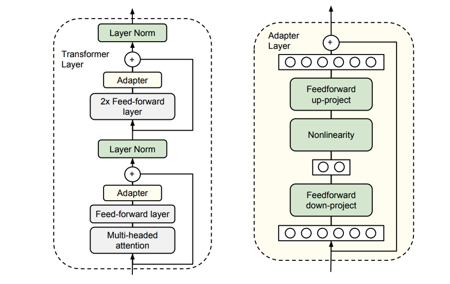
Model (adapter) only add a few trainable parameters per task compared with fine-tuning top-layers
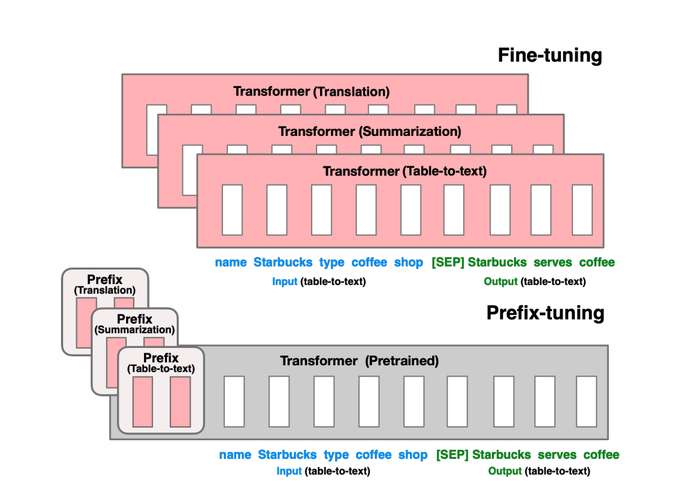
Model (prefix tuning) optimize a small continuous task-specific vectors (i.e. prefix)
Model (LoRA, low rank adaptation) constraining the updated parameter to be low-rank
where \(B,A\) has much lower rank
Model (T-few) multiplies activations with learned vectors
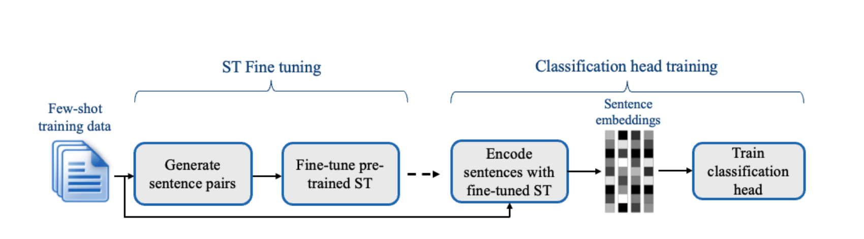
Model (setfit) two stage adaptation
- contrastive fine-tuning
- head training
Model (hypernet) use a smaller network to generate weight for a larger network, weights of small network are learned