0x004 Matrix
- 1. Foundation
- 2. Triangular Matrix and Equivalence
- 3. Diagonal matrix and Similarity
- 4. Unitary, Normal Matrix and Unitary Equivalence, Similarity
- 5. Hermitian, Symmetric Matrix and Congruence
- 6. Positive Semidefinite, Positive Definite Matrix
- 7. Tensor Analysis
- 8. Reference
This section only treats matrix and finite dimension vector, other related notes are
- finite-dimension vector space, operator is covered in 0x011 Linear Algebra
- infinite-dimension Banach space, Hilbert space is covered in 0x023 Functional Analysis
- numerical linear algebra is covered in 0x311 Numerical Linear algebra
1. Foundation
1.1. Subspace
Definition (fundamental subspace) There are four fundamental subspaces in linear algebra
- \(N(A)\): null space of A
- \(C(A)\): column space of A
- \(N(A^T)\): null space of \(A^T\)
- \(C(A^T)\): row space of \(A\)
The Big Picture of Linear Algebra Gilbert Strang
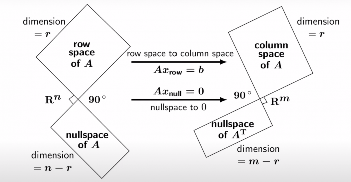
Lemma (dimension of fundamental subspaces) - The dimension of \(C(A)\) is the number of pivot (also equals \(rank(A)\)) - The dimension of \(N(A)\) is the number of free variables.
Therefore, we have the fundamental theorem of linear algebra as follows:
And similarly,
Lemma (orthogonal fundamental subspaces) Null space \(N(A)\) is orthogonal to row space \(C(A^T)\), therefore
And similarly,
Proof: Intuitively, for any vector \(x\) such that \(Ax=0\), \(x\) is orthogonal to every row in \(A\), therefore any linear combination from row space is also orthogonal to \(x\). In other words, \(Ax = 0\) implies for all \(y\), \((y^T A)x = 0\), therefore, \(y^TA\) and \(x\) are orthogonal.
null and column space are not always orthogonal
Unforunately, even the matrix is square, null space and column space might not be orthogonal. Consider the matrix
Both column space and null space are spanned by \((1,0)\)
1.2. Rank
Definition (rank) rank is the dimension size of the column space
Lemma (inequalities of rank) For any \(A,B,C\) with the same shape,
If \(A,C\) is nonsingular, then
1.3. Trace and Determinant
Lemma (cyclic permutation properties) Trace has a cyclic permutation property useful to compute derivatives
Lemma (inequalities determinant) The following inequality is known as the Hadamard's inequality
1.4. Exponential
This is a summary from the wikipedia page
Definition (exp) the matrix exp is defined as
This series converges for all \(X\), therefore well-defined
application in ODE
The solution of
is given by
Lemma (properties) It is easy to see
- \(\exp(YXY^{-1}) = Y\exp(X)Y^{-1}\)
- \(XY=YX \implies \exp(X+Y) = \exp(X)\exp(Y)\)
Theorem (trace identity)
Theorem (Golden-Thompson inequality)
computing
When $X$ is diagonalizable, $X = UAU^-1$, then by the previous property, we can compute
When \(N\) is nilpotent, we can sum the finite series
In a more general case, we transform \(X\) into Jordan canonical form and apply exponential to each Jordan block which can be written as \(\lambda I + N\) where \(N\) is nilpotent
1.5. Derivatives
Annoyingly, there are two types of vector and matrix layouts:
- the numerator layout (consistent with the Jacobian)
- the denominator layout (consistent with the Hessian).
They are transpose of each other. Note that the standard chain rule is consistent with the numerator layout, it also changes its order in denominator layout.
A easy rule to distinguish these two is to check its shape. Suppose \(x \in \mathbb{R}^{a \times b}, y \in \mathbb{R}^{c \times d}\), the most general tensor shape is as follows
Definition (numerator layout) The numerator layout has the shape
Definition (denominator layout) The denominator layout has the shape
when \(a,b,c,d\) is 0, it might be dimension reduced to simplify notation. For example, when \(x,y\) is a column vector (i.e, \(b,d = 0\)), when denominator layout is simplified to \((c,a)\) instead of \((c,1,a,1)\)
In the ML community, it looks the latter are more commonly used, so this section is follows the denominator layout.
Be careful this are all tranposed in the Jacobian matrix.
Under this layout, some important conclusions are
\(tr(BA)\) can be seen as the inner product of two matrix \(\langle B, A \rangle\), the following one is easy to see by noticing its similarity with \(\langle x, a \rangle\)
Theorem (Jacob's formula)
This has a special as case follows:
Corollary (Determinant's derivative)
Proof can be obtained by expanding det with cofactor. Here is a pdf containing its proof
This slide is also very good
application
Combined with the concavity of \(\log\det\), we can apply the first order condition to obtained an upperbound of \(\log\det X\)
1.6. Submatrices
A simple rule inverse of triangular submatrix is as follows
A more general inverse rule is to use schulr's complement. it is used, for example, to compute conditional probability and marginalized probability in multivariable normal distribution.
Definition (schur's complement) Schur's complement of the block matric
is defined to be
Theorem (partitioned inverse formula) The inverse of the original matrix
Derivation of this formula is to apply Gaussian elimination, details can be found in this lecture note or MLAPP 4.3.4.1
This can be applied to give the matrix inversion, it might reduce the complexity
Corollary (Sherman-Morrison-Woodbury)
If the shape of matrix \(A\) is \(N \times N\), matrix \(D\) is \(D \times D\), then the LHS has \(O(N^3)\) and RHS has \(O(D^3)\), this is helpful when \(N >> D\)
Special case of Sherman-Morrison-Woodbury
The previous form is the most general form of the inversion formula. There are several special cases of it worth noticing
1-rank pertubation:
1.7. Norm
A norm is a function that assigns a real-value length to each vector. A norm must satisfy
first, we review the vector norm, these are all special cases of general p-norm with counting measure
Definition (p-norm) the p-norm are defined below
the most common p-norms are
There are some relations between those norms, for example
Theorem (Holder inequality) Let \(1/p+1/q=1\), then
Cauchy Schwartz
Cauchy-Schwarz inequality is a special case of Holder's inequality
Norms arise naturally in the study of power series of matrices and in the analysis of numerical computations
For example, it is sufficient to say the following formula is valid when any matrix norm of \(A\) is less than 1
Intuitively, the matrix norm is to give the upper bound of range vector, intuitively, this is the maximum factor by which \(A\) can stretch a vector \(x\).
Note that the matrix norm is also a special case of the operator norm.
Definition (induced matrix norm) Given vector norms \(|| \cdot ||_{(n)}\) and\(|| \cdot ||_{(m)}\) on the domain and the range of \(A\), the induced matrix norm \(||A||_{(m,n)}\) is the maximum factor by which \(A\) can stretch a vector \(x\)
In particular, we can consider following special induced norms:
1-norm
Definition (1-norm of a matrix) If \(A\) is any \(n \times n\) matrix, then \(||A||_1\) is equal to the "maximum column sum" of \(A\)
2 norm
Definition (2-norm spectral norm)
\(\infty\) norm
Definition (\(\infty\) norm of a matrix) The \(\infty\) norm of an \(m \times n\) matrix is equal to the "maximum row sum"
The matrix does not need to be induced, in the general form, it will be defined as:
Definition (generalized matrix norm) The matrix norm is a function \(|| \cdot || \to \mathbf{R}\) that must satisfy the following properties:
- \(||\alpha A|| = |\alpha| ||A||\)
- \(||A+B|| \leq ||A|| + ||B||\)
- \(||A|| \geq 0\)
In the case of square matrices, it has to satisfy the following property.
Definition (Frobenius norm) Frobenius norm is to think of matrix as a long vector and to take vector norm.
It can also be written using the singular values
Proof \(\|A\|_F = \sum_{i,j} (a_{i,j})^2 = tr(A^T A) = \sum_i \lambda_i = \sum_i \sigma_i^2\)
This norm can also be derived from the Frobenius inner product, where we define the inner product of two matrices
Definition (nuclear norm) Nuclear norm is the dual norm of spectral norm
Nuclear norm is related to low rank approximation. It is used in the Netflix Prize. According to this paper. Minimization of the nuclear norm, NNM, is often used as a surrogate (convex relaxation) for finding the minimum rank completion (recovery) of a partial matrix.
The minimum nuclear norm problem can be solved as a trace minimization semidefinite programming problem, SDP. Interior point algorithms are the current methods of choice for this class of problems
numpy API for norms
numpy has norm library for all of those matrix norms
a = np.array([[1,2],[0,2]])

# Fro norm by default
np.linalg.norm(a) # 3.0

# nuc norm
np.linalg.norm(a, 'nuc') # 3.61

# 1 norm
np.linalg.norm(a, 1) # 4.0

# 2 norm
np.linalg.norm(a, 2) # 2.92

# inf norm
np.linalg.norm(a, np.inf) # 3.0
1.8. Inverse
Criterion (invertible) The following conditions characterize the invertible matrix \(A\) equivalently
- \(rank(A)=n\)
- \(range(A) = R^n\)
- \(null(A) = \{ 0 \}\)
- \(0\) is not eigenvalue
- \(0\) is not singular value
- \(det(A) \neq 0\)
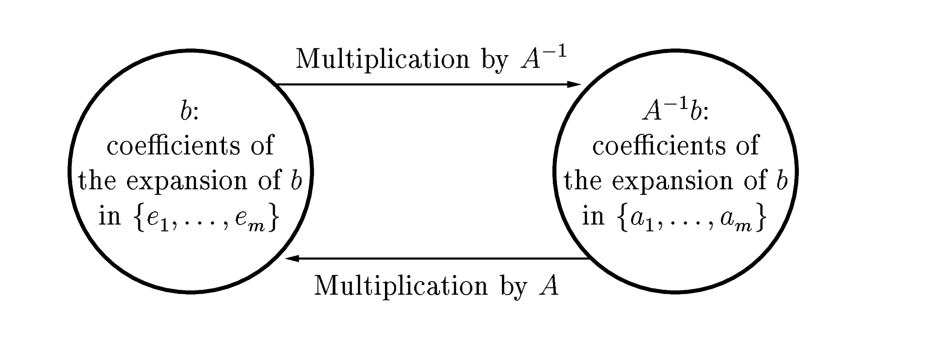
An invertible matrix can be used to change basis: \(A^{-1}b\) is the coefficients of the expansion of \(b\) in the basis of columns of \(A\).
Definition (generalized inverse) Let \(A \in R^{m \times n}\) be any matrix, we call the matrix \(G \in R^{n \times m}\) a generalized inverse of \(A\) if
Note if \(A\) is square and invertible, then the ordinary inverse \(A^{-1}\) is the only generalized inverse
generalized inverse might not be unique
Consider \(A = [1, 2]\), its generalized inverse can be any vector \(G=[x, y]\) such that
Therefore, there are many possible generalized inverse, e.g: \([1, 0], [3, 1]\)
Algorithm (construction, existence of generalized inverse) Let \(A = [[A_{11}, A_{12}], [A_{21}, A_{22}]] \in R^{m \times n}\) a matrix of rank \(r\), if \(A_{11} \in R^{r \times r}\) and invertible, then the following is a generalized inverse
Any matrix can be re-arrange into this form by row, column permutation, which proves the existence of generalized inverse
construction example
Consider the matrix
it has rank 2, we take the left 2x2 matrix and reverse it to be
The Moore-Penrose inverse is a special case of generalized inverse with more constraints, check this slide for more distinction
Definition (Moore-Penrose inverse, pseudo-inverse) a pseudoinverse of \(A\) is defined as a matrix \(A^+\) satisfying the following conditions:
- \(AA^+A = A\)
- \(A^+AA^+ = A\)
- both \(AA^+, A^+A\) are Hermitian
\(A^+\) exists for all matrix \(A\) and is unique. Construction of pseudo-inverse can be classified into two cases depending on the rank
Algorithm (full rank construction) When the matrix has full rank, we can explicitly compute \(A^\dagger\) use either or both of the following approach.
- \(A^\dagger = (A^*A)^{-1}A^*\) when \(A\) has linearly independent columns, this is called left inverse
- \(A^\dagger = A^*(AA^*)^{-1}\) when \(A\) has linearly independent rolws, this is called right inverse
Algorithm (non-full rank construction) One approach to get pseudo inverse is using SVD
where the form is the reduced form SVD. Other approach is also possible (e.g: CR decomposition)
application
\(A^\dagger b\) is a solution of the least squares problem
when the solution is not unique, \(A^\dagger b\) gives the solution with minimum norm.
2. Triangular Matrix and Equivalence
2.1. Row Reduction
Definition (row equivalence) Two matrices \(A,B\) of the same shape are said to be row equivalent
iff they share the the same row space or null space
Row equivalence can be established by applying a sequence of elementary row operations.
Definition (elementary row operation) The followings are elementary row operations
- swap: swap two rows
- scale: scale 1 row by nonzero constant
- pivot: add a multiple of 1 row to another row
matrix form of row operation
Each of the elementary row operation is corresponding to a invertible matrix form.
swap example: swap row 1 and row 2
scale example: scale row 3 by 5 times
pivot example: add 4*row 1 to row 3
Lemma (properties of row equivalent matrix) It is easy to show that
- A matrix is invertible if it is row equivalent to identity matrix
- rank is perserved (because null space is same)
Note that eigenvalues, vectors are not preserved.
The most "canonical" form of row equivalent matrix is the echelon form and reduced echelon form
Definition (echelon form, reduced echelon form) A matrix is in echelon form if it satisfies the following properties
- All nonzero rows are above any rows of all zeros
- each leading entry of a row is in a column to the right of the leading entry of the row above it
- all entries in a column below a leading entry are zeros
Intuitively, this means the nonzero leading entry has a steplike pattern in the matrix.
Note that each matrix may be row reduced into more than one echelon forms.
Definition (reduced echelon form, row canonical form) In addition to the echelon conditions, it also has to satisfy:
- the leading entry in each nonzero row is 1
- each leading 1 is the only nonzero entry in its column
Note that each matrix can be row reduced into 1 form of echelon matrix, so this is the canonical form with respect to row equivalence.
With the reduced echelon form, we can define pivot
Definition (pivot) A pivot position in a matrix \(A\) is a location in \(A\) that corresponds to a leading 1 in the reduced echelon form of \(A\). A pivot column is a column of \(A\) that contains a pivot position.
pivot variables and free variables
Consider the following echelon form linear system
The leading unknowns in the system \(x_1, x_3, x_4\) are called pivot variables, the other unknowns, \(x_2, x_5\) are called free variables.
Collorary (algebra of triangular matrix) Triangular matrix is preserved under many operations. For example,
- sum of upper triangular is upper triangular
- product of upper triangular is upper triangular
- inverse (if exists) of upper triangular is upper triangular
Decomposition (LU decomposition) Sometimes a matrix can be decomposed into two triangular matrix by recording steps in Gaussian elimination, when we eliminating row \(j\) using row \(i\) with a multiplier
and row operation
The multipliers can be tracked with the lower triangular matrix \(L\)
Be careful the multiplers' sign are reversed.
The LU decomposition is not always applicable, for example, the following permutation matrix
can not be LU decomposed.
We need PLU decomposition where \(P\) is a permutation matrix
application of LU decomposition
LU decomposition is useful to solve \(Ax = b\), expecially for a fixed A and a sequence of different \(b\), by decomposing \(A = LU\), we can solve \(L(Ux) = b\) by solving the following two equation efficiently
2.2. Linear System
This subsection is about solving linear equation
where we reduce \(A\) into echelon form through a series of row operations.
Note that if \(b=0\), this system is called homogeneous
Definition (consistency) A linear (or nonlinear system of equations) is called consistent if it has at least 1 solution (it might have infinitely many solutions); otherwise it is called inconsistent
Definition (overdetermined system) A system of equations is called overdetermined if it has more equations than unknowns. It can be either consistent or inconsistent (though usually inconsistent)
consistent case of overdetermined systems
The following overdetermined equation is a consistent example.
Definition (exact determined system) A system of equations is called exact-determined if the number of unknowns is equal to the number of equations. It also can be consistent or inconsistent.
Definition (underdetermined system) A system of equations is called underdetermined if it has more unknowns than equations. Again, it can be consistent or inconsistent (though usually consistent)
inconsistent case of underdetermined systems
The following underdetermined equation is an inconsistent example
Criterion (consistency) The following three are equivalent iff criterion of consistency.
- \(b\) is in the column space of \(A\).
- \(A\)'s rank is equal to the rank of augmented matrix \([A,b]\).
- the right most column of the augmented matrix is not a pivot column (e.g: echelon form of the augmented matrix has no row of the form \([0, ..., 0, b]\) with \(b\) nonzero)
Note the 3rd statement basically says if there is such a row, then appending \(b\) will result in 1 more rank.
Algorithm (size of solution set) To decide how many solutions we have, we should
- first, apply the previous consistency condition to check whether it is feasible
- if feasible, then check the null space of the matrix (or its rank), the dimension of solutions set is the dimension of null space.
2.3. Equivalence
Equivalent matrices represent the same linear transformation V → W under two different choices of a pair of bases of V and W, with P and Q being the change of basis matrices in V and W respectively
Definition (matrix equivalence) two rectangular matrix \(A,B\) are called equivalent if
for some invertible matrix \(P,Q\).
It can be seen as obtaining \(B\) by applying a sequence of row and column operations to \(A\).
Definition (canonical form) Every \(m \times n\) matrix is equivalent to a unique block matrix of the form:
where \(r\) is its rank.
equivalence vs similarity
similarity is a special case of equivalence and is much more restrictive:
- equivalence is defined wrt two invertible matrix, it can be non-square
- similarity is defined wrt 1 invertible matrix, and has to be square
3. Diagonal matrix and Similarity
3.1. Eigenvalue and Eigenvector
Definition (eigenvalue, eigenvector) An eigenvector of an \((n, n)\) matrix \(A\) is a nonzero vector \(x\) such that
A scalar \(\lambda\) is called an eigenvalue of \(A\) and \(x\) is called an eigenvector corresponding to \(\lambda\)
When \(\lambda\) is an eigenvalue, then the null space of \(A - \lambda I\) is nontrivial and we have a name for it.
Definition (eigenspace) The eigenspace of \(A\) corresponding to \(\lambda\) is all solutions of
Definition (spectrum) The spectrum of \(A \in M_n\) is the set of all \(\lambda \in C\) that are eigenvalues of \(A\); denoted by \(\sigma(A)\)
A diagonalizable matrix can be represented in the following form
where \(\Lambda\) is a diagonal matrix \(diag(\lambda_1, ..., \lambda_n)\), \(X\) is a matrix whose columns are eigenvectors \(x_i\)
Because columns of \(X\) are linear independent and \(X\) spans the whole space, \(X\) is invertible, and we obtain the following decomposition.
Decomposition (eigen-decomposition, diagonalization)
An diagonalizable matrix \(A\) can be factorized into the following form
This decomposition can be interpreted clearly by considering component.
If \(v=\sum_i c_i x_i\), Multiplying \(X^{-1}\) is to extract the coefficient component under the basis of \(X\)
Multiplying \(A\) is to extend linearly each eigenvector by eigenvalue.
Then using the original basis to represent the vector by multiplying \(X\)
With this decomposition, we can compute \(A^k\) efficiently by
In particular, if \(\lambda < 1\), it can be dropped when \(k\) is large enough.
3.2. Similarity
This section is to study of similarity of \(A \in M_n\) via a general nonsingular matrix \(S\): the transformation \(A \to S^{-1} A S\)
Similar matrices are just different basis presentations of the same linear transformation, similar matrices have the same set of eigenvalues (spectrum) and characteristic polynomial.
Diagonalizable matrices have independent eigenvectors, but not necessarily orthogonal.
Similar matrices represent the same linear map under two (possibly) different bases, with P being the change of basis matrix
Definition (similarity) \(A, B \in M_n\). We say that \(B\) is similar to \(A\) if there exists a nonsingular \(S \in M_n\) such that
Similarity is an equivalence relation on \(M_n\), sometimes we write \(A ~ B\) to express similarity.
Corollary (Invariant under similarity) There are several properties preserved by the similarity relation.
- rank
- eigenvalues (however, same set of eigenvalues does not imply similarity because multiplicity also need to be preserved)
- characteristic polynomial
- Jordan Normal Form
3.3. Jordan Canonical Form
Recall equivalence yields same canonical form, but similarity yields the Jordan Normal Form
Diagonalization is a special case of Jordan Normal Form
Definition (diagonalizable) If \(A \in M_n\) is similar to a diagonal matrix, then \(A\) is said to be diagonalizable
Note that \(P,D\) are not unique and \(D\) might not be diagonal matrix of eigenvalue and \(P\) might not be eigenvectors.
Note that diagonalizable matrix does not require orthonormal basis.
Criterion (eigenspace) A \(n \times n\) matrix is diagonalizable if and only if eigenspace spans the whole space (eigenspace dim is \(n\))
defective matrix is not diagonalizable
A defective matrix is a matrix does not have a basis of eigenvector (therefore not diagonalizable). A example is a shear matrix
Criterion (distinct eigenvalue) A useful sufficient condition is to check the unique eigenvalue, if there are \(n\) distinct eigenvalue, then the matrix is diagonalizable (because eigenvalue of each eigenvector are independent and thus spans the whole space)
Note the converse is not true.
converse case
Consider the identity matrix \(I_2\), it is obviously diagonalizable.
It has only 1 eigenvalue (1), but the eigenspace has 2 dimension, therefore diagonalizable.
Lemma (sum of rank-1 matrices) A diagonalizable \(A \in M_n\) can be decomposed into sum of \(n\) rank-1 matrices
where \(x_i\) is the (right) eigenvector, \(y_n\) is the left eigenvectors of \(A\) (i.e.: \(y^T A = \lambda y^T\))
4. Unitary, Normal Matrix and Unitary Equivalence, Similarity
analogous to a number \(r\) where \(|r|=1\)
Definition (unitary matrix, orthogonal matrix) A matrix \(U \in M_n\) is unitary if \(U U^* = I\). A matrix \(U \in M_n(R)\) is real orthogonal if \(U^T U = I\)
The set of unitary matices in \(M-n\) forms a group \(U(n)\) which is a subgroup of \(GL(n)\).
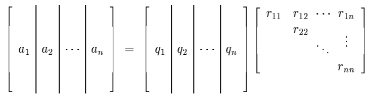
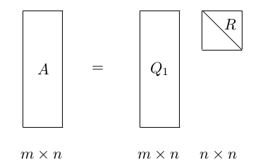
4.1. QR Decomposition
Decomposition (QR decomposition) Decomposition of a matrix into a orthogonal matrix and a triangular matrix \(\(A = QR\)\)
where \(Q\) is the orthogonal matrix and \(R\) is the upper triangular matrix.
It can be illustrated as follows:
Note that it is an enhanced version of CR decomposition with Gram-Schmit
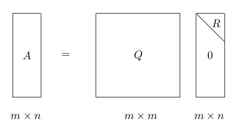 A reduced thin version of QR is also available
4.2. Unitary Similarity
Unitary similarity is a special case of similarity
Definition (unitary similarity) \(A\) is unitarily similar to \(B\) if there exists a unitary matrix \(U\) such that
Definition (unitary diagnolizability) We say that \(A\) is unitarily diagonalizable if it is unitarily similar to a diagonal matrix
4.3. Normal Matrices
Definition (normal matrix) A matrix \(A \in M_n\) is called normal if \(A\) commutes with its conjugate transpose
Example: A diagonalizable matrix might not be a normal matrix
Theorem (statements of normal matrix) Let \(A= [ a_{ij} ] \in M_n\) have eigenvalues \(\lambda_1, ..., \lambda_n\). The following statements are equivalent
- \(A\) is normal
- A is unitarily diagonalizable
- \(\sum_{i,j=1}^n |a_{ij}|^2 = \sum_i^n |\lambda_i|^2\)
- \(A\) has \(n\) orthonormal eigenvectors.
4.4. Unitary Equivalence and SVD
Recall the equivalence is defined as follows:
Definition (equivalence) Two matrices are said to be equivalent iff there exist invertible matrices \(P,Q\) such that
Notice similarity is defined to use the same matrix for transformation., but equivalence is using two matrix for transformation.
Unitary equivalence is defined as follows:
Definition (unitary equivalence) For \(A \in M_{n,m}\), the transformation \(A \to UAV\) in which \(U \in M_n,V \in M_m\) are both unitary, is called unitary equivalence
Recall from Linear Algebra: in the abstract vector space. Suppose for an operator \(T \in \mathcal{L}(V)\). The singular value of \(T\) are defined to be eigenvalues of the positive operator \(\sqrt{T*T}\).
Suppose \(T\) has singular values \(s_1, ..., s_n\). Then there exist orthonormal bases \(e_1, ..., e_n\) and \(f_1, ..., f_n\) of \(V\) such that
The statement of SVD under finite-dimension is: every matrix \(A\) is diagonal \(\Sigma\) when one uses proper bases for the domain \(V\) and range \(U\) spaces, where \(V\) is corresponding to the orthonormal bases \(e_1, ..., e_n\) and \(U\) is corresponding to \(f_1, ..., f_n\)
Decomposition (Singular Value Decomposition) Let \(A \in M_{n,m}\) matrix with rank r, there exists a matrix \(\Sigma \in M_{n,m}\) where the diagonal entries are nonegative ordered values: \(\sigma_1 \geq \sigma_2 ... \geq \sigma_r \geq 0\), and orthogonal matrix \(U \in M_{n,n}\), \(V \in M_{m,m}\) such that
The form is (orthogonal) x (diagonal) x (orthogonal), most importantly the diagonal matrix \(\Sigma\) has the same shape as \(A\). Note that the decomposition (orthogonal) x (diagonal) x (orthogonal) would not be unique without restricting the nonnegative ordered values on the \(\Sigma\). (e.g: \((-U) (-\Sigma) V^T\))
The reduced form of SVD using rank \(r\) can be written as
This decomposition can also be written in the rank 1 sum form
\(u_i, v_i\) are left and right eigenvectors, they are connected with \(A\) by
In the matrix form, it is
Corollary (range and null from SVD) The range and null space can be easily identified with the SVD decomposition
This is actually the most accurate approach to find orthonormal basis for range and null space.
Theorem (existence of SVD) Every matrix is diagonal, provided one uses the proper bases for the domain and range spaces.
Proof: See Trefethen Bau P29. \(\sigma_1 = ||A||_2\) is determined by the compactness, therefore we can find unit vector \(u_1, v_1\) such that \(Av_1 = \sigma_1 u_1\). Extending \(u_1, v_1\) to \(U_1, V_1\), we can decompose \(U_1^*AV_1\) into a simpler matrix, then apply the induction.
Theorem (uniqueness of SVD) The singular values \(\{ \sigma_i \}\) are uniquely determined. If \(A\) is square and \(\sigma_i\) are distinct, the left/right singular vectors \(\{ u_i \}, \{ v_i \}\) are uniquely determined up to complex signs
Proof: By contradiction, if not singular vector are not unique, then singular values are not simple.
Note if singular values are not unique, then there are freedoms chosing orthonormal basis among the subspace sharing the same singular value. See this slide for more details.
non-unique SVD
If \(\sigma_i\) is not simple (i.e: there are two identical singular value), then there are some freedom to chose the orthonormal spaces, for example
where \(\theta\) can be any number.
Theorem (Eckart-Young) The first k rank 1 sum is the best rank \(k\) approximation of \(A\), suppose that \(B\) has rank k, then
singular value VS eigenvalue
Note that singular value does not match eigenvalue in general, actually the first singular value is the upper bound.
However, in some cases, they could be identical, for example.
If \(S=Q\Lambda Q^T\) is symmetric positive definite matrix, then \(U=V=Q\) and \(\Sigma=\Lambda\)
If \(S\) is symmetric but has negative eigenvalue, then the corresponding singular value is its reverse, and one set of the corresponding singular vector is its reverse.
On the application side - eigenvalue tend to be relevant to problems involving the behavior of the iterated forms of \(A\) (e.g: \(A^k, e^{tA}\)) - singular vectors tend to be relevant to problems involving the behavior of \(A\) itself or its inverse
SVD VS eigendecomposition
There are fundamental differences between SVD and eigendecomposition.
- SVD uses two different bases, but eigendecomposition only uses one (the eigenvectors)
- SVD uses orthonormal bases, but eigendecomposition might not be
- all matrices have a SVD, but eigendecomposition is not
Decomposition (Polar Decomposition) polar decomposition is analogous to \(re^{i\theta}\), where an arbitrary matrix \(A\) can be decomposed into an orthogonal matrix \(Q\) and symmetric positive semidefinite matrix \(S\)
4.5. Projection
Let's first consider projecting vector \(b\) into another vector \(a\). Supposed the projected vector is \(xa\) where \(x\) is a scalar, then it is clear \(b - xa \perp a\), therefore
Solving this formula, we know
Therefore, the projected vector is
or equivalanetly
where \(\frac{aa^T}{a^Ta}\) is a rank 1 matrix acting on \(b\)
These formulas can be simplified using unit vectors. Notice if we normalized \(a\) into \(q=a/||a||\), then the projected vector is simply
which computes the length \(b^Tq\) first and multiplies it to \(q\). The projected vector can also be written equivalently as
where \(q^Tq\) is a rank 1 matrix, which acts on \(b\).
Instead of projecting a vector \(b\) into a vector spans by a single vector \(a\), we can generalize this idea into projecting \(b\) into the column space spanning by a matrix \(A\).
First we would define what matrix is qualified as the projection matrix
Definition (Projection) A square matrix is called a projector if it satisfies
The projection is said to be idempotent because any higher power than 1 does not change results (another example is closure)
properties of projection matrix
The eigenvalue of a projection \(P\) over space \(E\) is either \(\lambda = 1\) or \(\lambda = 0\).
The eigenspace of 1 if \(ker(P)\) and eigenspace of 0 is \(ker(I-P)\) where \(E = ker(P) \oplus ker(I-P)\)
The trace of \(P\) is its rank
Definition (complementary projection) If \(P\) is a projection, then \(I-P\) is called the complementary projection. It is also a projection because
The projection and complementary projection can be connected by range and null, where
The projection is equivalent to split the space into two disjoint subspace \(S_1, S_2\), where \(S_1\) is corresponding to the range, and \(S_2\) is corresponding to the null space. Note in this case, \(S_1, S_2\) are not required to be orthogonal. When they are not orthogonal, it is called the oblique projection.
When they are orthogonal, we have the orthogonal projection. A matrix is an orthogonal projection if
Theorem (orthogonal projection) A projector \(P\) is orthogonal if it is hermitian
Algorithm (projection with orthonormal basis) when projecting to the column space of an orthonormal basis matrix \(Q\), the projection matrix \(P\) can be written as
In the column-wise representations,
Notice the similarity with the previous discussion of \((qq^T)b\), instead of taking a single rank 1 matrix, this is taking a sum of rank 1 matrix.
The more general projection with arbitrary basis is as follows.
Algorithm (projection with generalized inverse) Let \(A\) be an m,n matrix, for any vector \(v\), suppose the projected vector is \(y\), then \(y-v\) should be orthogonal to range A, therefore \(A^*(y-v)=0\), because \(y \in \mathrm{range}(A)\), then \(y=Ax\) for a \(x\), \(A^*(Ax - v)\) becomes
\(x\) can be solved by
and the projection \(P\)
We can easily verify that this \(P\) satisfies the projection properties (e.g: \(P^2=P\))
Again notice the similarity with the previous discussion where projection into a dim 1 vector space is
5. Hermitian, Symmetric Matrix and Congruence
analogous to a real number
Definition (hermitian conjugate, adjoint) The hermitian conjugate or adjoint of an \(m \times n\) matrix \(A\), written \(A^*\), is the \(n \times m\) matrix whose \(i,j\) entry is the complex conjugate of the \(j, i\) entry of \(A\)
Definition (hermitian) A matrix is called hermitian iff
A hermitian matrix has to be, by definition, square.
Definition (symmetric) If a real matrix is hermitian, it is says to be symmetric.
Theorem (eigen-decomposition, spectral theorem) The eigen-decomposition of a symmetric matrix is as follows:
In an equivalent form, it can be represented by a rank 1 symmetric matrix sum
proof
Theorem (eigenvalues of symmetric matrix are real)
suppose \(Ax = \lambda x\), then \(\bar{x}^TAx = \lambda \bar{x}^Tx\)
Additionally, \(\bar{A}\bar{x} = \bar{\lambda} \bar{x} \implies \bar{x}^T A = \bar{\lambda} \bar{x}^T \implies \bar{x}^TAx = \bar{\lambda} \bar{x}^Tx\), so we know \(\lambda = \bar{\lambda}\)
Theorem (eigenvector of symmetric matrix are orthogonal)
Suppose \(Sx = \lambda x, Sy = \alpha y\), then\(y^T S x = \lambda y^T x\), \(x^T S y = \alpha x^T y\) and \(y^T S x = x^T S y\). therefore \(\lambda - \alpha x^T y = 0\) and \(x^T y = 0\) when \(\lambda \neq \alpha\)
Interestingly, there is also a "reversed" version of hermitian: skew-hermitian
Definition (skew-hermitian) A matrix is called skew-hermitian iff
It is easy to prove that eigenvalues of skew-hermitian matrix are all imaginary
5.1. Congruences and Diagonalizations
Definition (*congruence, T-congruence) Let \(A,B \in M_n\), if there exists a nonsingular matrix \(S\) such that
Then \(B\) is said to be *congruent or conjunctive to \(A\). If
Then \(B\) is said to be T-congruent to \(A\)
Note that both types of congruence are equivalence relations.
Theorem (Sylvester's law of inertia) Congruent matrices have the same number of positive, negative, zero eigenvalues
6. Positive Semidefinite, Positive Definite Matrix
analogous to a non-negative, positive number. It is corresponding to the positive operator in linear algebra.
Definition (positive definite, positive semidefinite) A Hermitian matrix \(A \in M_n\) is positive definite if for all nonzero \(x \in C^n\)
It is positive semidefinite if for all nonzero \(x \in C^n\)
6.1. Characterizations and Properties
Property All entries on diagonal of Hermitian positive semidefinite matrix are positive.
Theorem (eigenvalue criterion) A Hermitian matrix is positive semidefinite iff all of is eigenvalues are nonnegative, it is positive definite iff all of its eigenvalues are positive.
Theorem (Sylvester's criterion) Let \(A \in M_n\) be Hermitian
- If every principal minor of \(A\) is nonnegative, then \(A\) is positive semidefinite
- If every leading principal minor of \(A\) is positive, then \(A\) is positive definite.
Decomposition (Cholesky decomposition) Cholesky decomposition is the decomposition of the following form where \(L\) is a lower triangular matrix with real and positive diagonal entries
Note that this is to find the square root
7. Tensor Analysis
7.1. Decomposition
Tensor is much more difficult to decompose
Decomposition (CP Decomposition) Approximate a given tensor \(T\) by a sum of rank one tensors \(A,B,C\)
This is a NP-hard problem, but can be computed in a reasonably efficient way by alternatively improve \(A,B,C\)
Decomposition (Tucker Decomposition) \(\(T \approx \sum_{p=1}^{P} \sum_{q=1}^{Q} \sum_{r=1}^{R} g_{pqr} a_p \circ b_q \circ c_r\)\)
where \(a,b,c\) are three sets of orthonormal columns.
8. Reference
- [1] Horn, Roger A., and Charles R. Johnson. Matrix analysis. Cambridge university press, 2012.
- [2] Golub, G. H. (1996). CF vanLoan, Matrix Computations. The Johns Hopkins.
- [3] Petersen, K. B., and M. S. Pedersen. "The Matrix Cookbook, vol. 7." Technical University of Denmark 15 (2008).
- [4] Strang, Gilbert. Linear algebra and learning from data. Wellesley-Cambridge Press, 2019.
- [5] Dan Margalit, Joseph Rabinoff. Interactive Linear Algebra
- [6] Murphy, Kevin P. Machine learning: a probabilistic perspective. MIT press, 2012.