0x531 Sequence

Using a standard network model (e.g: MLP model to predict output concats with input concats) to represent sequence is not good, we have several problems here

• inputs, outputs length can be variable in different samples
• features learned at each sequence position are not shared
• too many parameters

2.1. RNN

The Vanilla RNN has the following architecture (from deeplearning ai courses)

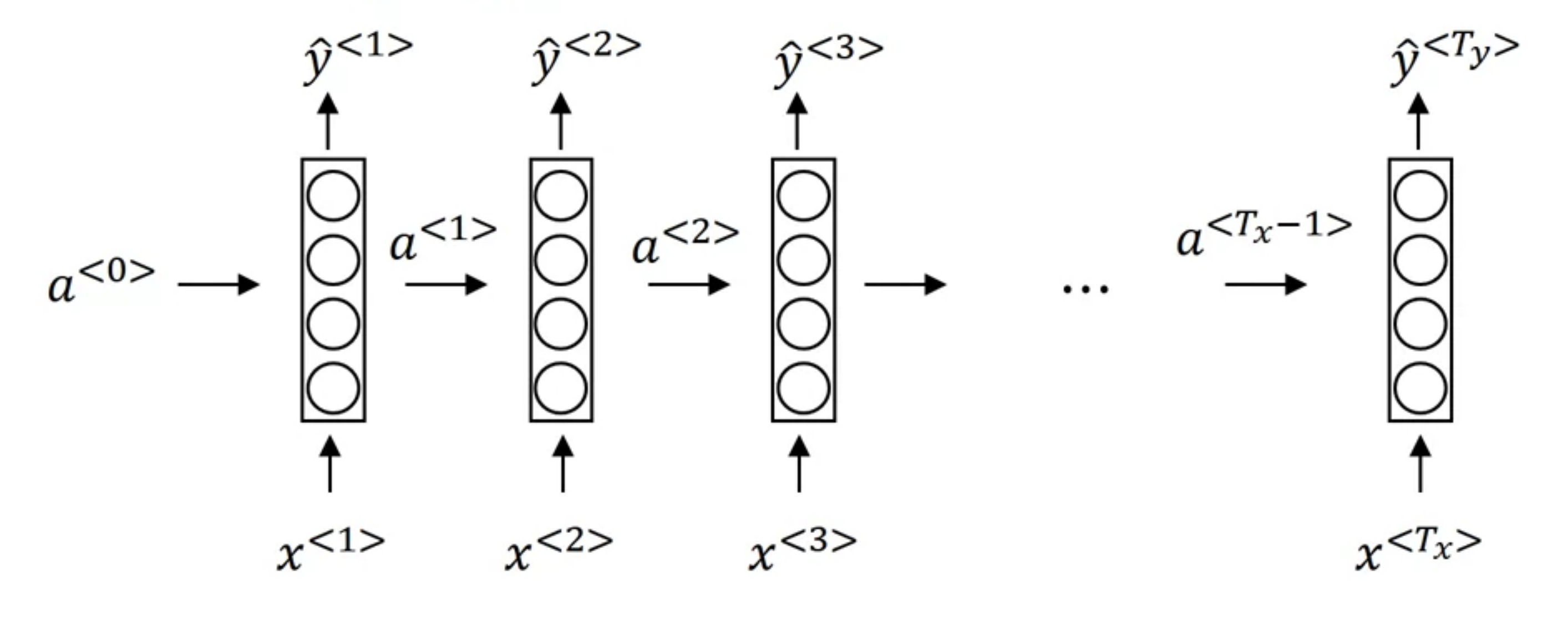
The formula are

\[h_{t+1} = \sigma(W_{rec} h_t + W_{in} x_t) = \sigma (W [h_t, x_t])\]

\[y_{t} = \sigma(W_{out} h_t)\]

2.1.1. Bidirectional RNN

This unidirectional vanilla RNN has some problem, let's think about an example of NER from the deeplearning.ai course.

• He said Teddy Roosevelt was a great president
• He said Teddy bears are on sale

It is difficult to make decision at the word Teddy whether it is a person name or not without looking at the future words.

2.1.2. Gradient Vanishing/Explosion

RNN has the issue of Gradient Vanishing and Gradient Explosion when it is badly conditioned. This paper shows the conditions when these issues happen:

Suppose we have the recurrent structure

\[h_t = W_{rec} \sigma(h_{t-1}) + W_{in} x_t\]

And the loss \(E_t = \mathcal{L}(h_t)\) and \(E = \sum_t E_t\), then

\[\frac{\partial E_t}{\partial \theta} = \sum_{1 \leq k \leq t} \frac{\partial E_t}{\partial h_t} \frac{\partial h_t}{\partial h_k} \frac{\partial h_k}{\partial \theta}\]

the hidden partial can be further decomposed into

\[\frac{\partial h_t}{\partial h_k} = \prod_{t \geq i \geq k} \frac{\partial x_i}{\partial x_{i-1}} = \prod_i W^T_{rec} diag(\sigma'(h_{i-1}))\]

Suppose the nonlinear \(\sigma'(h_t)\) is bounded by \(\gamma\), then \(|| diag(\sigma'(h_t)) || \leq \gamma\) (e.g: \(\gamma = 1/4\) for sigmoid function)

It is sufficient for the largest eigenvector \(\lambda_1\) of \(W_{rec}\) to be less than \(1/\gamma\), for the gradient vanishing problem to occur because

\[||\frac{\partial h_{t+1}}{\partial h_{t}}|| \leq ||W_{rec}|| ||diag(\sigma'(h_t))|| < 1\]

Similarly, by inverting the statement, we can see the necessary condition of gradient explosion is \(\lambda_1 > \gamma\)

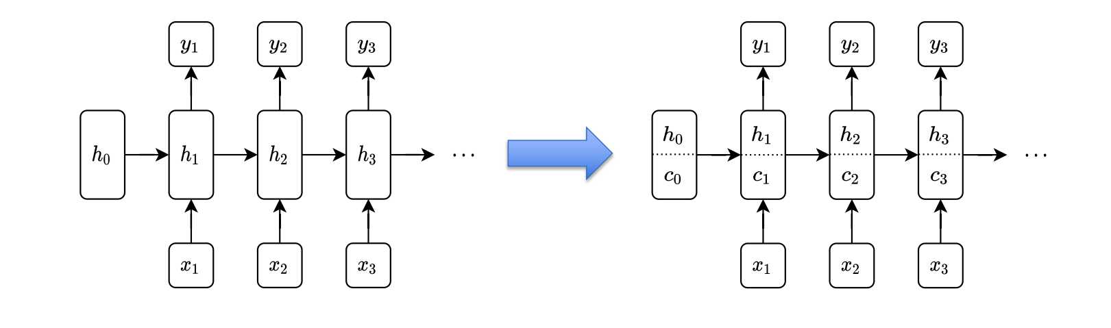
2.2. LSTM

Model (LSTM) Avoid some problems of RNNs

It computes the forget gates, input gate, output gates

\[\begin{bmatrix} i_t \\ f_t \\ g_t \\ o_t \end{bmatrix} = \begin{pmatrix} \sigma \\ \sigma \\ tanh \\ \sigma \end{pmatrix} (W_{hh} h_{t-1} + W_{hx} x_t + b_h)\]

The following one is the key formula, where the saturating \(f_t \in [0,1]\) will pass grad through \(c_{t}\) to \(c_{t-1}\)

\[c_t = c_{t-1} \circ f_t + i_t \circ g_t\]