0x503 Reinforcement Learning

• 1. Value Approximation
  • 1.1. Linear Model
  • 1.2. Model-based Methods
  • 1.3. Model-free Methods
• 2. Reward Approximation
  • 2.1. Demonstration
  • 2.2. Human Feedback
• 3. Policy-based Model
  • 3.1. Policy Gradient Theorem
  • 3.2. Monte Carlo Policy Gradient (REINFORCE)
    • 3.2.1. Advantage function
    • 3.2.2. Convergence
  • 3.3. Actor-Critic
  • 3.4. Deterministic Policy Gradient
    • 3.4.1. DPG
    • 3.4.2. DDPG
  • 3.5. Policy Optimization
    • 3.5.1. TRPO
    • 3.5.2. PPO

The problems of tabular based approach in classic RL are: (as mentioned in (Sutton and Barto, 2018)¹)

• it has large number of state spaces, which requires large memory and computation
• in many tasks, almost every state encountered will never have been seen before

We would like to use approximated models to generalize our observations.

1. Value Approximation

This section estimate the state-value function from on-policy data, following Chapter 9 of (Sutton and Barto, 2018)¹

First, We use approxmiated value-function models parameterized with \(w\):

\[\hat{v}(s; w) \approx v_\pi(s)\]

\[\hat{q}(s, a; w) \approx q_\pi(s,a)\]

The objective is

\[\overline{VE}(w) = \sum_{s \in \mathcal{S}} \mu(s)[v_\pi(s) - \hat{v}(s; w)]\]

Typically, the number of weights \(w\) is much less than the number of states.

Then we update \(w\) using MC or TD learning

1.1. Linear Model

1.2. Model-based Methods

AlphaGo[silver2016mastering] has a few training stages

• stage 1: supervised learning training two policy networks: \(p_{\pi}(a | s)\) for faster rollout linear policy and \(p_{\sigma}(s | a)\) for accuate SL policy
• stage 2: instantiate RL policy network \(\rho\) with \(\sigma\) and improve by gradient policy
• stage 3: learn state value function \(v\) from policy \(\rho\)

During search, it uses Monte Carlo Tree Search (MCTS) to search

• selection: action is selected based on \(Q\) and an exploration bonus \(u\)
• when expanded, it selects action based on \(\rho\) and store action distribution
• simulation is done towards end using faster rollout \(\pi\)
• evaluation is done by combining simulation and value function \(v\)
• backup is is standard count-based backup

AlphaGo Zero (Silver et al., 2017)² improves from AlphaGo by purely self-playing with no supervision or human data

In AlphaGo Zero, policy network and value network are combined into one network \((p, v) = f_\theta(s)\). The objective is to try to match policy \(p\) with MCTS search probability \(\pi\)

MCTS is done as follows:

• select edge with \(Q(s,a)+U(s,a)\) recursively until the leaf node where \(U(s,a) \propto P(s,a)/(1+N(s,a))\)
• the leaf node is expanded by \((P, V) = f_\theta\) and \(P\) get stored
• backup is done by \(Q(s,a) = 1/N(s,a) \sum_{s'} V(s')\)

During self-play, search probability \(\pi_a \propto N(s,a)^{1/\tau}\) where \(\tau\) is temperature.

At the end of self-play, a reward \(r_T\) is assigned and intermediate outputs \((s_t, \pi_t, z_t)\) where \(z_t = \pm r_T\) are collected as training data.

The objective is to try to match policy \(p\) with search probability \(\pi\) and \(v\) with \(z\) for each \(s_t\)

AlphaZero (Silver et al., 2018)³ further generalizes AlphaGo Zero by replacing winning probaility with expected outcome and removes game-specific assumptions (e.g. data augmentation from game-specific invariance).

1.3. Model-free Methods

Model (DQN) proposed in Playing Atari with Deep Reinforcement Learning (Mnih, 2013)⁴ is an classic example of Q-Learning method.

DQN's highlights are the following two strategies to stablize training.

experience reply:

• it stores experience \(e_t = (s_t, a_t, r_t, s_{t+1})\) into buffer
• a minibatch is sampled from buffer in every iteration for backprop

fixed Q target: compute Q-learning wrt to old parameters \(w^-\)

DQN's input is raw pixels, output is a value function estimating future rewards for each action (note output here is reward for each action, not policy (action distribution))

MuZero

2. Reward Approximation

Recall reward depends on state and action \(R(s,a)\), to declaratively define a good reward might be difficult.

In deep RL, we want to learn reward function instead

2.1. Demonstration

In typical RL, we learn \(\pi\) from \(R\), but here we learn \(R\) from \(\pi\)

Model (inverse RL) inverse RL is defined to be the problem of extracting a reward function given observed optimal behavior.

Suppose we know the state, action space and transition model. Given a policy or demonstrations, we want to find reward \(R\)

Here is a lecture slide

Offline IRL is to recover the rewards from a fixed, finite set of demonstrations.

Model (max entropy) recover the reward function by assigning high rewards to the expert policy while assinging low rewards to other policy based on the max entropy principle

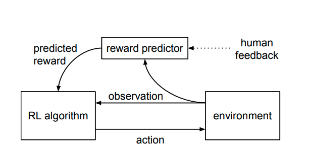
2.2. Human Feedback

Model (human preference model) solving tasks that human can only recognizes the desired behavior instead of demonstrating it

The reward is first trained using human ranking instead of ratings.

Those rewards are fed to the RL algorithm

3. Policy-based Model

Policy based algorithm learns a good policy \(\pi\), which should generate actions that produce good reward (e.g: REINFORCE). It does not depend on value functions.

\[\pi_\theta(a | s) = P(a | s, \theta)\]

Learning \(\pi_\theta(s,a)\) instead of \(Q_\theta(s,a)\) might result in more compact representation. For example, we do not need to estimate the exact score in \(Q\). (analogy to diff between discrminative and generative approach)

Another advantage is it allows continuous action space. For example, we can sample continuous action from a normal distribution parameterized by mean, var from \(\pi_\theta\). See this [Q.A](https://datascience.stackexchange.com/questions/37434/policy-based-rl-method-how-do-continuous-actions-look-like

Other Advantages:

• directly optimize the objective function
• local convergence
• learn useful stochastic policies (e.g: optimal policy of iterated rock-paper-scissors game is uniform random: Nash equilibrium)
• sometimes policy are simple while models and value are complex

Disadvantage:

• high variance
• sample inefficiency

3.1. Policy Gradient Theorem

How do we measure the quality a policy \(\pi_\theta\)?

• In episodic environment, we can use the start value

\[J(\theta) = v_{\pi_\theta}(s_0)\]

• In continuing environment, we can use average value where \(d^{\pi_\theta}(s)\) is stationary distribution of Markov chain

\[J(\theta) = \sum_s d^{\pi_\theta}(s) v^{\pi_\theta}(s)\]

Policy Gradient Theorem simplifies the gradient of performance wrt parameter that does not involve derivative of the state distribution. In the episodeic case, we have

\[\nabla J(\theta) \propto \sum_s \mu(s) \sum_a q_\pi(s, a) \nabla \pi(a, s| \theta)\]

where \(\mu\) is the on-policy distribution under \(\pi\). In the expectation form, it is

\[\nabla J(\theta) = \mathbb{E}_{S_t \sim \pi} [\sum_a q_\pi(S_t, a) \nabla \pi(a, S_t| \theta)]\]

Applying gradient-ascent to this results in

\[\theta_{t+1} = \theta_t + \alpha \sum_a {\hat{q}(S_t, a) \nabla \pi(a | S_t, \theta)}\]

where \(\hat{q}\) is some learned approximation to \(q_\pi\).

This algorithm is called an all-action method because its involving all of the actions by taking sum.

3.2. Monte Carlo Policy Gradient (REINFORCE)

MC policy gradient or REINFORCE simplifies the all-action method by taking sample from action space. It first rewrite

\[\begin{eqnarray}\nabla J(\theta) &=& \mathbb{E}_{S_t \sim \pi} [\sum_a q_\pi(S_t, a) \nabla \pi(a | S_t,\theta)] \\ &=& \mathbb{E}_{S_t \sim \pi} [\sum_a \pi(a | S_t, \theta) q_\pi(S_t, a) \frac{\nabla \pi(a | S_t, \theta)}{\pi(a | S_t, \theta)}] \\ &=& \mathbb{E}_{S_t, A_t \sim \pi} [q_\pi(S_t, A_t) \frac{\nabla \pi(A_t | S_t, \theta)}{\pi(A_t | S_t, \theta)}] \\ &=& \mathbb{E}_{\tau \sim \pi}[G_t \nabla \log \pi(A_t | S_t, \theta)] \end{eqnarray}\]

The last equation is done by \(\mathbb{E}_\pi[G_t | S_t, A_t] = q_\pi(S_t, A_t)\)

By sampling the episode, we update REINFORCE:

\[\theta_{t+1} = \theta_t + \alpha G_t \nabla \log \pi(A_t | S_t, \theta)\]

The following REINFORCE algorithm snippet is from (Sutton and Barto, 2018)¹

The key idea here is during learning, actions that result in good outcomes should become more probable. These actions are positively reinforced. Actions are changed by following the policy gradient:if the return \(G_t > 0\), then the probability of the action \(\pi_\theta(a_t | s_t)\) is increased, otherwise it is decreased

3.2.1. Advantage function

To reduce the variance of the REINFORCE, one approach is to normalize the reward as

\[\nabla J(\theta) \approx \sum_{t=0}^T (G_t - b(s_t)) \nabla_\theta \log \pi(A_t | S_t, \theta)\]

where \(b(s_t)\) might be the value function \(V\), this is related to the Actor-Critic algorithm. Another option is to use the mean over the trajectory

\[b = \frac{1}{T} \sum_t G_t\]

the function which is the discounted rewards minus a baseline is called the advantage function

3.2.2. Convergence

There are several works dealing global convergence of policy gradient methods:

• LQR

3.3. Actor-Critic

The REINFORCE algorithm suffers the variance in the gradient estimation, which requires large samples to train. To improve this

we combine both value function and policy Based models in Actor-Critic Method

• an actor is a policy-based method, it controls how our agent behaves \(\pi_\theta(s)\)
• a critic is a value-based method, it measures how good the taken action is, \(\hat{q}_w(s, a)\)

3.4. Deterministic Policy Gradient

Deterministic policy gradient is the limiting case of stochastic policy gradient when policy variance tends to zero.

3.4.1. DPG

DPG paper

3.4.2. DDPG

3.5. Policy Optimization

The vanilla policy gradient is hard to hard to choose step sizes because

• input data (e.g. episode) is non-stationary due to changing policy
• bad step is more damaging than in supervised learning

3.5.1. TRPO

TPRO (Trust Region Policy Optimization)

Constraining the gradient update using KL-divergence

3.5.2. PPO

PPO (Proximal Policy Optimization)

PPO also improves the training stability by avoid taking too large policy updates

watch this lecture

---

1. Richard S Sutton and Andrew G Barto. 2018. Reinforcement learning: An introduction. MIT press. ↩↩↩

2. David Silver, Julian Schrittwieser, Karen Simonyan, Ioannis Antonoglou, Aja Huang, Arthur Guez, Thomas Hubert, Lucas Baker, Matthew Lai, Adrian Bolton, et al. 2017. Mastering the game of go without human knowledge. nature, 550(7676):354–359. ↩

3. David Silver, Thomas Hubert, Julian Schrittwieser, Ioannis Antonoglou, Matthew Lai, Arthur Guez, Marc Lanctot, Laurent Sifre, Dharshan Kumaran, Thore Graepel, et al. 2018. A general reinforcement learning algorithm that masters chess, shogi, and go through self-play. Science, 362(6419):1140–1144. ↩

4. Volodymyr Mnih. 2013. Playing atari with deep reinforcement learning. arXiv preprint arXiv:1312.5602. ↩