0x411 Classical Model
- 1. Linear Classification Model
- 2. Dimension Reduction
- 3. Clustering
- 4. Kernel Methods
- 5. Tree Model
- 6. Markov Random Field
- 7. Recommendation System
- 8. Reference
The ML probabilistic model can be largely grouped into two models: generative model and discriminative model. The former models the joint distribution \(p(x,y)\) and the latter models the posterior distribution \(p(y|x)\). Andrew Ng's famous paper suggests the following points when comparing generative models
- generative model has a higher asymptotic error than discrminative model
- generative model approach this asymptotic error much faster, with \(O(log(N))\) samples vs \(O(N)\) samples.
Model (Generative Model) Generative Model is to model the joint distribution \(P(\textbf{x}, \textbf{y})\).
This typically can be broken into modelling of conditional distribution and probability distribution:
- models a class conditional densities \(P( \textbf{x} | y=y_k)\)
- models a class prior \(P(y=y_k)\)
With the joint distribution, the prediction task is easily solve with posterior distribution. - compute posterior \(P(y=y_k | \textbf{x})\) with Bayes' theorem
Generative model tends to be better when training data are limited, but the bound of the asymptotic error is reached more quickly by a generative model than a discriminative model. Additionally, it performs worse when the density assumption give a poort approximation to the true distribution.
Definition (Discriminative Model) The approach of a discriminative model is to model posterior distribution directly \(P(\textbf{y} | \textbf{x})\) directly.
For example, in the classification task, it is to model \(P(y=y_k | \textbf{x})\) directly
Parameters are typically estimated with MLE. for example, by iterative reweighted least squares (IRLS)
Discriminative model tends to achieve better results with asymptotic classification error (when training data are large enough)
Models that do not have probabilistic interpretation but can learn decision boundary are called discriminant function, these can also be classified as the (nonprobabilistic model) discriminative model. For example, SVM. These directly assigns each vector \(x\) to a specific class.
1. Linear Classification Model
Definition (classification task) The goal of classification is to take an input vector \(\textbf{x}\) and assigned it to one of \(K\) discrete classes \(\mathcal{C_k}\)
Definition (decision region, decision boundary) The input space is divided into decision regions whose boundaries are called decision boundaries
1.1. Discriminant Functions
Model (two class) In the case of two classes, we assign to \(C_1\) if \(y \geq 0\), otherwise \(C_0\)
the decision boundary is \(y = 0\), which is a hyperplane
For any point \(x\), the signed distance to the hyperplane is
When \(x\) is at the origin, it reduced to \(r = -w_0/||w||\)
Definition (K class) In the case of multiclasses, we create a single \(K\)-class discriminant comprising \(K\) linear functions of the form
where we assgin a point \(\mathbf{x}\) to \(\mathcal{C}_k\) if \((\forall j \neq k) y_k(\mathbf{x}) > y_j(\mathbf{x})\)
The decision regions are connected and convex
1.1.1. Fisher's Linear Discriminant
Note this is slightly different from the previous LDA.
Suppose two classes of observations have means \(\mu_0, \mu_1\) and covariance \(\Sigma_0, \Sigma_1\). Fisher defined the separation between two distributions to be the ratio of the variance between the classes to the variance within the classes.
It can be shown the maximum separation occurs when
1.1.2. The perceptron algorithm
Proposed by Rosenblatt [2]. Minsky's work analyzes perceptron [3].
The perceptron learns a threshold function to map its input \(x\) to an output \(f(x)\)
The criterion is given by
Intuitively, the critrion is trying to match the sign of \(t_i\) and \(w^Tx\).
By applying the gradient descent, the \(w\) can be updated by
where \(\gamma\) is the learning rate.
Convergence:
- When linear separable, perceptron converges in finite steps, upper-bounded by \(\frac{R^2}{\gamma^2}\) where \(R\) is the upper-bound of norm of training set \(x\). The solution and convergence typically depends on the initial value. proof of this statement
- When not linear separable, it will never converge
1.2. Generative Model
The general Gaussian Discriminative Analysis (GDA) is to model the class conditional densities with multivariate Gaussian distribution
If there is no assumption about the \(\Sigma_k\), then it is known as quadratic discriminant analysis (QDA), which is literally a quadratic classifier (because of \(\Sigma\))
GDA has two simplifications: Naive Bayes and Linear Discriminative Analysis.
1.2.1. Naive Bayes
If the \(\Sigma_k\) is diagonal, this is equivalent to the Naive Bayes classifier.
Naive bayes is based on the assumption that features \(\mathbf{x}\) are mutually independent given the output \(\mathcal{C}_k\) (i.e. \(y=k\)). The joint probability distribution is modeled as follows
1.2.2. Linear Discrimative Analysis
When \(\Sigma_k\) in GDA are shared or tied across all classes (i.e.: \(\Sigma_k = \Sigma\)), then it is known as the linear discrimative analysis (LDA) \(\(p(y=k | x) \propto \exp (\mu_c^T \Sigma^{-1} x -\frac{1}{2} \mu_c^T \Sigma^{-1} \mu_c + \log \pi_c)\)\)
It is called linear because the exponent can be expressed in linear with respect to \(x\)
LDA can be solved analytically with MLE
1.3. Discriminative Model
Advantage of discrminative models is that it has fewer adaptive parameters which may lead to improved predictive performance
1.3.1. Logistic Regression
The logistic regression has the probabilistic form
and
The negative log-likelihood for logistic regression is given by
This is called the cross entropy loss function
Taking derivative of this, we derive
By computing Hessian of this function, we know
Therefore, the objective is convex and has a unique global minimum.
1.3.1.1. Max Entropy
maximize the entropy of joint distribution
with the feature constraint of \(E_p f_j = E_{p^{~}} f_j\)
1.3.1.2. Logistic Regression vs Naive Bayes
The hypothesis space of Gaussian Naive Bayes and Logistic Regression is same: each parameter of Logistic Regression is corresponding to a set of Gaussian Naive Bayes parameters. (i.e. every Gaussian Naive Bayes can be mapped to a logistic regression model)
In gaussian naive bayes, we have \(\(p(y=1 | x) = \frac{p(x|y=1)p(y=1)}{p(x|y=1)p(y=1)+p(x|y=0)p(y=0)} = \frac{1}{1+exp(-a)}\)\)
where
However, the general Gaussian Naive Bayes cannot be represent with logistic regression, for example, decision boundary of Gaussian Naive can be curved, but logistic regression cannot. When Naive Bayes has the same covariance across all classes, then they have the same form.
See Andrew Ng's paper for asymptotic convergence comparison.
1.4. Maximum Margin Classifier (SVM)
One of the limitation of the kernel methods is that the kernel function \(k(x_n, x_m)\) must be evaluated for all possible pairs \(x_n, x_m\). In this section, we look at kernel-based algorithms that have sparse solutions.
Consider the linear model \(y(x) = w^T \phi(x) + b\), and label \(t \in \{ 1, -1 \}\)
Recall the perpendicular distance of a point \(x\) from a hyperlane defined by \(y(x)=0\) is given by
1.4.1. Separable Case: Hard SVM
In the case of linear separatable dataset such that for all \(n\), we have \(t_n y(x_n) > 0\), this \(t_n y(x_n)\) can also be seen as a confidence score to classify this data point correctly. we want to maximize the margin to the closest point
Comparing SVM with perceptron, it looks that perceptron is maximizing the total margin, but the SVM is maximize the margin to the closest point.
Direct solution of this problem is difficult, we scale \(w, b\) such that nearest point satisfies \(t_n(w^t\phi(x_n) + b)=1\) and all points satisfy the constraints
and the original problem is to minimze \(||w||^2\), which is now a quadratic programming problem.
To solve this, we write the Lagrangian
Solving the KKT condition gives
where the last term is the complementary condition. A vector \(x_i\) with \(\alpha_i \neq 0\) is called support vectors, which satisfies \(y_i (w^T x_i + b) = 1\). Note while the solution \(w\) is unique, but support vectors are not.
Using KKT condition, the dual optimization problem becomes
subject to
This is again a QP problem because Hessian of objective function is PSD
This once again can be solved by both general-purpose or specialized QP solver (e.g SMO algorithm)
1.4.2. Non-separable Case: Soft SVM
2. Dimension Reduction
Check this lecture note
2.1. Global Distance Preservation
This group preserves pairwise distance among all datapoints
Model (PCA) There are two equivalent formulation of PCA
- maximize the variance of projected data
- minimize the error of data and their projections
In the maximum variance formulation, we consider the projection one to a unit direction of \(u_1\). Each point \(x_n\) is projected to \(u_1^Tx_n\). The variance of projected data is
where \(S=\sum_{i=1}^N (x_i-\bar{x})(x_i-\bar{x})^T/N\) is the data covariance matrix
Solving this with the constraint \(u^Tu = 1\) using Lagrange multiplier, we can see \(u_1\) is the eigenvector having the largest eigenvalue \(\lambda_1\), the eigenvalue is the variance: \(u_1^TSu_1 = \lambda_1\)
Projecting the top-\(M\) eigenspaces can be done using power method with \(O(MD^2)\) where \(D\) is \(S\)'s dimension
PCA is a projection from one dataset (one multidimension variable), A closely related concept wrt two datasets (two multidimensional variables) is CCA
Model (CCA, canonical corelation analysis) Given two random variables \(X=(x_1, ..., X_n), Y=(y_1, ..., y_m)\) from two datasets, we might want to analyze their correlation, however, computing \(pq\) correlation ratios are not intuitive, so we want to summarize into a few statistics.
To achieve this, we iteratively project \(X,Y\) into \(U_k=a_k^TX, V_k=b_k^TY\) such that maximizing their correlation \(\rho = corr(U_k, V_k)\) but kept new projected direction to be uncorrelated with previous direction (i.e \(cov(U_k, U_1) = 0, cov(V_k, V_1)=0\))
check this tutorial
2.2. Local Distance Preservation
Model (t-SNE)
Model (UMAP, Uniform Manifold Approximation and Projection) check its tutorial doc
3. Clustering
Clustering is the process of grouping similar objects together.
There are two kinds of inputs we might use
- similarity based clustering: the input to the algorithm is an \(N \times N\) distance matrix or dissimilarity matrix matrix \(D\)
- feature-based clustering: the input is an \(N \times D\) feature matrix or design matrix \(X\).
There are also two kinds of outputs we might expect:
- flat clustering (partitional clustering): we partition the objects into disjoint sets
- hierarchical clustering: we create a nested tree of partitions
3.1. Partitional Clustering
3.1.1. Spectral Clustering
Spectral clustering make uses of spectrum of the similarity matrix to perform dimension reduction before clustering in fewer dimension. In application to image segmentation, spectral clustering is known as segmentation-based object categorization.
This tutorial has the full treatment of this topic. The following is a summary from the tutorial.
The basic idea of spectral clustering is to use graph cuts: find a partition of the graph such that
- the edges between different groups have a very low weight
- the edges within a group have high weight
Formally, we want to find a partition into \(K\) clusterings \(A_1, ..., A_k\) such that
where \(W(A,B) = \sum_{i \in A, j \in B} w_{ij}\)
Unfortunately, this often partitions off a single data point from the rest. To ensure the sets are reasonably large, we use the normalized cut as the objective
where \(vol(A) = \sum_{i \in A} d_i\)
To find the optimal assignment binary vector \(c = [c_1, ..., c_K]\), however, is NP-hard. We can relax the binary to be real-value and solves it as an eigenvector problem.
We first create a sparse matrix \(W\) from the similarity matrix \(S\) by
- only keeping edge whose distance is less than \(\epsilon\)
- for each vertex, only keeping the \(K\) nearest neighbor connections
Then we create the Graph Laplacian \(L\)
where \(D\) is the degree matrix (i.e. the diagonal matrix with the degrees d1,...,dn on the diagonal.) and \(W\) is the adjancecy matrix
There are a couple of important properties of Graph Laplacian, for example, it is a PSD matrix with \(0\) as the smallest eigenvalue.
and most importantly
proposition (Number of connected components and the spectrum of L) Let \(G\) be an undirected graph with non-negative weights. Then the multiplicity \(k\) of the eigenvalue 0 of \(L\) equals the number of connected components \(A_1,...,A_k\) in the graph. The eigenspace of eigenvalue 0 is spanned by the indicator vectors \(\mathbf{1}_{A_1} ,..., \mathbf{1}_{A_k}\) of those components
See the section 3.1 of tutorial for the proof
This suggests the following algorithm
Input: Similarity matrix S \in R^{n x n}, number of k cluster
- Construct the weighted adjacency matrix W from S
- compute the Graph Laplacian L
- compute the k eigenvectors (corresponding to the k smallest eigenvalues) u_1, ..., u_k
- Let U = [u_1, ..., u_k] be a new feature matrix where each row y_i \in R^k is the feature for point i
- run k-means on the new feature matrix and fine the k clusters
There are two normalized version of Graph Laplacian
The symmetric matrix
The random matrix
Both are highly related to the original problem and can be solved using similar approaches.
3.2. Hierarchical Clustering
Semi-supervised Learning
Model (LGC, Learning with Local and Global Consistency) label propagation (from labeled data to unlabeled data) over graph affinity matrix \(W\) with smooth regularization.
4. Kernel Methods
There is a class of ML which stores the entire training set in order to make predictions for future data points. This are called the memory-based methods or instance-based methods.
They typically require a metric to be defined that measures the similarity (i.e.: kernel function) of any two vectors in input space.
4.1. Kernel Functions
To construct valid kernel functions, one approach is to choose a feature space mapping \(\phi(x)\) and use it to find the kernel
An alternative approach is to construct kernel functions directly (e.g: \(k(x,z) = (x^Tz)^2\)), but we need to make sure this kernel is a valid kernel
Condition (valid kernel) A necessary and sufficient condition for a function \(k(x,x')\) to be a valid kernel is that for all possible \(x_n\), Gram matrix \(K\) should be positive definite.
Some commonly used kernel family
radial basis function, alsown known as the homogeneous kernels, depends only on the magnitude of the distance
stationary kernel, which are invariant to translations
4.2. Kernel SVM
Extending the linear SVM optimization and solution, we obtain
The hypothesis solution \(h\) is
with \(b = y_i - \sum \alpha_j y_j K(x_j, x_i)\) for any \(x_i\) with \(0 < \alpha_i < C\)
It turns out that the fact that SVM's solution can be written as a linear combination of \(K(x_i, )\) is not unique to SVM, it is a general property that holds for a broad class of optimization problems
Theorem (representer) Let \(K\) be a PDS kernel and \(H\) its corresponding RKHS, then for any non-decreasing regularization function \(G\) and any loss function \(L\), the optimization problem
admits a solution of the form
4.3. Sequence Kernel
5. Tree Model
5.1. CART (Classification and Regression Tree)
The decision tree models are defined by recursively partitioning the input space, and defining a local model (e.g: a constant) in each resulting region of input space. They are popular for several reasons.
Pros
- easy to interpret
- can handle discrete and continuous features
- insensitive to monotone transformation (scaling)
Cons
- accuracy is not as good as other models
- high variance
5.1.1. Regression Trees
Regression Tree partitions the input space into \(M\) regions: \(R_1, ..., R_M\) and it models the response as a constant \(c_m\) in each region
The best partition is generally computationally infeasible, so we proceed with a greedy algorithm. The split at each step is selected on split variable \(j\) and split point \(s\), which partition the space into two half-planes:
The criterion is to minimize the square error
where \(\hat{c_1}, \hat{c}_2\) is the response average
To manage the complexity, the preferred strategy is to grow the tree into a large tree \(T_0\) (e.g: stopping the splitting only when some minimum node size (5) is reached). The from \(T_0\), we apply the pruning.
The complextiy criterion of a subtree \(T \subset T_0\) can be defined using hyperparameter \(\alpha\)
where \(|T|\) is the leaf count, \(Q_m\) is the leaf square error and \(N_m\) is the number of sample for leaf \(m\).
For each \(\alpha\), there is a unique optimal smallest subtree \(T_{\alpha}\), which can be found during the process of pruning the weakest link toward the root.
5.1.2. ID3 (Classification Trees)
ID3 is an algorithm by Ross Quilan in 1986. It recursively split the tree based on the Information gain. The splitting process is by greedy search (the optimal split is NP-hard)
There are three criterions to decide the split at each node: information gain, Gini impurity and misclassification error. Typically the first 2 are used to grow the tree and the last one is used to prune the tree.
Definition (information gain) Information gain is defined as follows
where \(H(S)\) is the entropy of parent node, \(A\) is the target splitting attribute, \(T\) is the subsets splitted by \(A\). Recall the entropy of a node is defined by
Definition (Gini impurity) Another splitting criterion is the Gini impurity, the impurtiy of a set is defined as
The split is selected by choosing the least weighted impurity (weighted by the size of the set).
Definition (misclassification error) Finally, a split criterion can be simply the error rate
5.1.3. C4.5, C5
These have some improvements from ID3 including
- can handle discrete (categorical feature) as well
- can handle missing values
C4.5 prunes the tree based on confidence interval of error rates, see the doc here
- we compare the upper limit error rate after pruning vs. average upper limit error rate before pruning
- if it reduces the upper limit error rate, we prune it
5.2. Ensemble
5.2.1. Adaboost
The motivation for boosting is to combine "weak" classifiers to produce a powerful "committee"
where \(\alpha_m\) is the weight for model \(G_m(x)\).
The procedure is roughly
- initialize all sample weight to \(w_i = 1/N\)
- fit a weak classifier \(G_m(x)\) to the weighted sample
- compute the weighted error rate
- use the error rate to compute the new model's weight
- use the new models' weight to update sample's weight exponentially
5.2.2. Gradient Boost
xgboost, lightgbm
5.2.3. Bootstrap Aggregation (Bagging)
As mentioned, the CART model is a high variance model. To reduce the vairance, we can apply the Bagging to ensemble \(n\) trees Typically, each tree receives a randomly chosen subset of the original data.
Unfortunately, simply rerun the same tree model will result in highly correlated predictors (which still results in high variance).
Random forest can decorrelate it by randomly choosing the subset of input variables for each node in each tree. Watch this video to see how RF works
6. Markov Random Field
A graphical model consists of the graph (structure) and statistical model (parameters):
- the graph encodes qualitative properties of the distribution
- the statistical model encodes the quantitative properties
The reason to use PGM:
- without graphical structure, configurations over high dimension will be exponential, which makes it difficult to learn and inference
- easy to integrate domain knowledge
- easy to integrate different models
undirected graphical model
We consider probability distribution over sets of random variables \(V = X \cup Y\) where \(X\) are input random variables and \(Y\) are output random variables. Given a collection of subsets \(A \in V\), we define an undirected graphical model as the set of all distributions that can be written in the form of
For any choices of factors \(F = \{ \Phi_A \}\) where \(\Phi_A: V^n \to R^+\)
The constant \(Z\) is called the partition function, which is a normalization factor
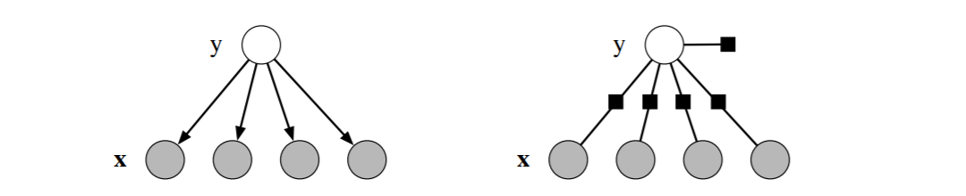
Graphically, this can be represented by a factor graph, which is a bipartite graph \(G=((V,F), E)\) where \(V\) is the set of variable nodes and \(F\) is a set of factor nodes: a variable \(v_s \in V\) is connected to a factor node \(\Phi_A \in F\) if \(v_s\) is an argument of \(\Phi_A\).
Each factor usually has the form
The right side of the following figure is the factor graph for Naive Bayes where the circles are variables nodes and boxes are factor nodes. (The left side is its Bayesian network representation)
6.1. Logistic Regression
Logistic regression is a discrminative model to predict a single class \(y\) based on a random vector \(\mathbf{x}\)
(or maximum entropy classifier in NLP) is motivated by the assumption that \(\log(y|x)\) is proportional to the linear function of \(x\). The conditional distribution is:
Feature functions are defined to be the indicator function \(f_{y', j}(x, y) = 1_{y' = y}(x_j)\)
When \(y\) is a binary class, normalization is simplified to
and it can be transformed into the sigmoid representation:
where \((\lambda_1-\lambda_0) + \sum_j (\lambda_{1, j}-\lambda_{0,j}) x_j\) are log odds
Notice this normalization over \(y\) is very easy to compute as there are only two options (\(y=1\) and \(y=0\)), however, in the more general CRF case, forward computing is necessary to normalize.
6.1.1. Maximum Entropy
The multinomial logistic regression is also known as the Maximum Entropy Classification model in the NLP literature. Check this book chapter
In the maximum entropy literature, the feature \(f_j(x)\) is usually a binary indicator. For each feature, we add a constraint to our distribution, specifying the our distribution should match the empirical distribution. Berger 1996 proposes a optimization problem to maximize entropy subject to those contraints. The solution to this problem has the form of the multinomial logistic regression.
See wikipedia for some derivation
6.2. Linear-CRF
See this blog
Linear-CRF generalizes the logistic regression to predict a sequence \(\mathbf{y}\) using a sequence \(\mathbf{x}\)
Let \(X,Y\) be random vectors, the linear-chain CRF is the distribution \(p(y|x)\) that takes the form
Notice this is a discriminative model which modeling the conditional probability \(p(y|x)\) directly
This particular linear-chain CRF implies the following conditional independence assumptions: each \(y_t\) is only dependent on its immediate predecessor \(y_{t-1}\) and successor \(y_{t+1}\) and \(\mathbf{x}\)
6.2.1. Estimation
The objective function is convex, so gradient descent is ok, but requires too many iterations. Better approaches are to approximate the second-order information such as LBFGS
6.2.2. Decoding
6.3. CRF
The general CRF further generalizes the linear CRF from a sequence structure to a more general graph structure
6.3.1. Estimation
Related materials:
6.3.2. Decoding
7. Recommendation System
7.1. Collaborative Filtering
Model (memory based approach) compute similarity between users or items. the similarity can be computed using Pearson correlation or cosine-similarity:
then we make predictions about the missing values
One drawback of the user-user and item-item approach is that they are not suitable for sparse matrix
Model (matrix decomposition) this approach aims to approximate the observed entries in \(X\) as a product of two lower-rank matrices
where \(U \in R^{m,k}, V \in R^{k,n}, k << m, n\)
\(U\) represents feature of each user, \(V\) represents feature of each item, the estimation is
The goal is to minimze the squarex loss function
which can be solved with the alternating least squares
Model (probabilistic matrix factorization) This is a probablistic version of the previous one, introducing prior to \(U, V\)
Model (Bayesian PMF) a fully Bayesian model of the previous one by further introducing hyperparameters
8. Reference
[1] CMU 10-708 lecture
[2] Stanford CS-228 lecture note
[3] introduction to CRF pdf
[4] Foundations of Machine Learning book