0x362 Database
- 1. History
- 2. Query Language
- 3. Index Management
- 4. Memory Management
- 5. Query Optimization
- 7. Reference
1. History
- 1960: Charles Bachman designed the Integrated Database System, the first DBMS. (Turing 1973)
- 1964: IBM designed IMS (hierarchical model) for Apollo program (BOM for Saturn V)
- 1969: CODASYL (network model) published
- 1970: Codd from IBM research lab published the paper of the relational model. (Turing 1981)
- 1973 Ingres project (led by Stonebraker) demostrate that it was possible to build practical and efficient implementation relation model. (Turing 2014)
- 1974: SQL designed by Donald Chamberlin and Raymond Boyce from IBM (SQL become ANSI standard in 1986)
- 1979: Oracle database
- 1995: MySQL (MySQL AB -> Sun Microsystems -> 2010 Oracle), it was forked into MariaDB by its cofounder.
- 1996: PostgreSQL (originally called POSTGRES from the Ingres database)
2. Query Language
2.1. Relational Algebra
Relational algebra defines the interface how to retrieve and manipulate tuples in a relation. Input is relation, output is relation, it is proposed by Codds when working in IBM.
Query (or expression) on set of relations produce relation as a result.
Note that semantics of relational algebra removes duplicates from relation when querying (because rows are set).
operator (selector) selector is to pick certain rows based on condition.
operator (project) project is to pick certain columns.
operator (cross product) combine two relations.
Suppose \(A\) has \(s\) tuples and \(B\) has \(t\) tuples, then cross product has \(st\) tuples. relation name is attached to each attribute to disambiguate.
operator (natural join) Enforce equality on all attributes with same name, and eliminate one copy of duplicate attributes.
Natural join does not add any expression power to algebra, it can be expressed using the join
operator (theta join) Apply the condition to join, this is the basic operation used in DBMS
The following are set operators operator (union) combines rows vertically, the schema should match
operator (difference)
operator (intersection) intersection can be expressed with union and difference
operator (rename) rename the schema for an relation
Rename operator is to unify schemas for set operators because schema must match.
2.2. SQL
SQL is the declarative language partially implementing the relational algebra, derived from SEQUAL from IBM. Row in SQL is an unordered multiset.
statement (select)
This is equivalent to the following sigma algebra
duplicates: select will return duplicate because SQL is a multiset model, to reduce the duplicates, add distinct after select
order: select will return results without any order, to force order, add order by attr at the end.
3. Index Management
An index is an additional structure that is derived from the primary data. Maintaining index incurs overhead, especially on writes.: well-chosen indexes speed up read queries, but every index slows down writes.
When the entire db cannot fit into the memory, we store them in the disk and maintain a index to map key into the disk offset. The following three are most common indexes, they can be kept on memory or disk.
3.1. Hash Index
Hash hash can be used as an in-memory index, one typical index is the following.
3.1.1. Bitcask
Bitcask is the default storage engine for Riak
This introduction paper is quite easy to understand.
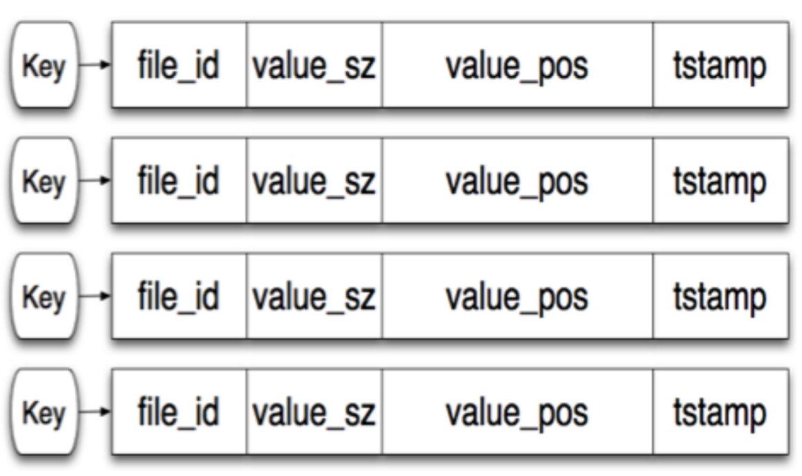
we use hash index to map the key to the offset of log-structured data file.
- Whenever we append a new key-value pair to the file, we update the hash point the key to the new offset.
- The logs are splitted into segments of a certain size, which would be compacted later.
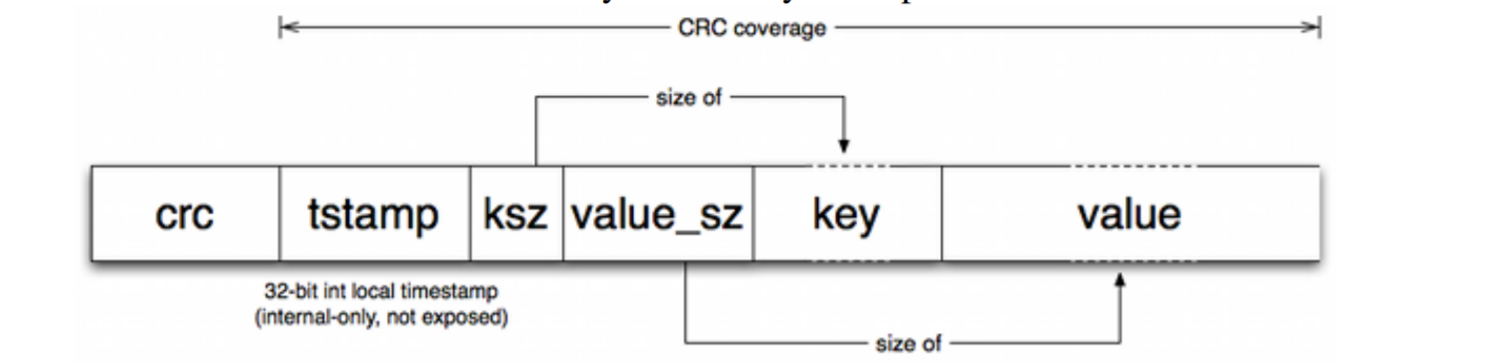
The hash map points to the file id (segment id), and its internal offset
The value field:
Pros:
- high speed read/write (the paper says it can do 5~6k writes per sec)
- good for case where the value for each key is updated frequently
Cons:
- entire hash map should be kept in memory
- range query are not efficient (might be achievable thorough secondary index though)
3.2. SSTable (memtable)
When we cannot fit entire hashmap into the memory, we can use SSTable or memtable
SSTable (e.g: red-black/AVL trees) is an in-memory index to store new key-value pairs
3.2.1. LSM-Tree and memtable
For even larger SSTable, we can write out some SSTable to storage and use memtable to only record the latest key-value pairs.
memtable (e.g: red-black/AVL trees) it stores new key-value pairs temporarily. When they gets bigger than some threshold (e.g: a few Mb), we write them sorted pairs into new SSTable.
Pros (over hash index):
- merging segments is simple and efficient using priority queue. (see this related Leetcode problem)
- in-memory index can be sparse: 1 key for every few kilo bytes. (because key-value are sorted in the segment)
Cons
3.2.2. LevelDB
3.2.3. Cassandra
3.3. B-Tree
4. Memory Management
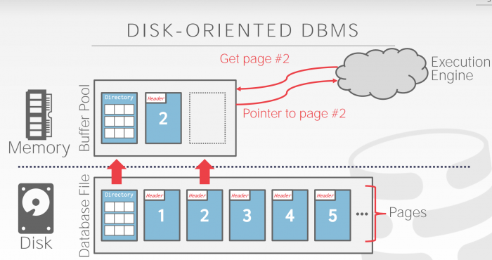
Buffer Pool is a large memory range as an array of fixed size pages. An array entry (slot) is called a frame. DBMS may have multiple buffer pools.
Page table keep tracks of pages that are currently in buffer pool, also maintains meta-data per page such as dirty flag, pin, reference counter for concurrency issue.
4.1. Optimization
- scan sharing: decide which page to evict based on access pattern of multiple queries
- pre-fetching: prefetch page based on query
- buffer pool bypass: bypass memory pool to reduce overhead
- OS page cache: O_DIRECT to bypass OS cache (one exception is postgre)
4.1.1. Buffer Replacement Policies
The followings are the most common policies. Enterprise db usually have much better policies than open source db
- LRU (Least Recently Used): maintain a timestamp, evict pages by timestamp order. The disadvantage of LRU is the sequential flooding for sequential scan, the most recent page is the most useless. clock: approximation of LRU, set to 1 when a page accessed, evict page whose when it is 0. Same problem as LRU
- LRU-K: take into account history of the last K references as timestamps and compute the interval between subsequent accesses, the interval helps to predict when the page will get accessed next time. Typical K is 1.
- Localization: restrict memory to its private buffer rather than polluting all memory.
- Priority Hints: provide hints whether a page is important or not. Dirty pages need to be taken account (e.g: background writing)
5. Query Optimization
Predicate Pushdown
Instead of applying filtering after loading all rows, Predicate pushdown push the filtering clause (e.g. WHERE) down to the source and reduce the transmission significantly.
5.1. Join Order and Algorithm
The performance of a query plan is largely determined by the order of join. Most query optimizers determine join order via a dynamic programming
To actually do the join, there are three join algorithms
Algorithm (nested loop join) nested two for loop for \(R\) and \(S\)
algorithm nested_loop_join is
    for each tuple r in R do
        for each tuple s in S do
            if r and s satisfy the join condition then
                yield tuple <r,s>
Algorithm (blocked nested loop) generalization of nested loop join. suppose \(|R| < |S|\). cache blocks of \(R\) in memory, only scan \(S\) 1 time for each block of \(R\)
Algorithm (sort-merge join) Sort \(R\) and \(S\) by the join attribute, then process them with a linear scan
Algorithm (hash join) building hash table (for the smaller relation), then probing the other table
7. Reference
- [1] Stanford Database Youtube Lectures
- [2] CMU Database Lectures
- [3] Kleppmann, Martin. Designing data-intensive applications: The big ideas behind reliable, scalable, and maintainable systems. " O'Reilly Media, Inc.", 2017.
- [4] Database Internals O'Reilly