0x043 Convex Optimization
1. Convex Sets
1.1. Affine Set
Definition (affine set) A set \(C \subseteq R^n\) is affine if for any \(x_1, x_2 \in C\), then \(\theta x_1 + (1-\theta)x_2 \in C\) where \(\theta \in R\)
note: Affine set is a subspace plus an offset
Definition (affine hull) The affine hull of \(C\) is the affine combination of all points in \(C\). The affine dimension of \(C\) is the dimension of its affine hull, which is the dimension of the underlying subspace
solution set of linear equations
The solution set of a system of linear equations is an affine set
hyperplane
A hyperplane is also a solution set of linear equation, therefore affine set
1.2. Convex Set
Definition (convex set) A set \(C\) is convex if for any \(x1,x2 \in C\), and any $0 \leq \theta \leq 1 $, then
Note the difference between affine set and convex set is the range of \(\theta\)
Definition (convex hull) The convex hull of \(C\) is the convex combination of all points in \(C\)
halfspace
A halfspace is a convex set
ball and ellipsoid
A norm ball is a convex set
A lreated family are ellipsoids, they are also convex
polyhedra and simplex
A polyhedron is defined as the solution set of a finite number of halfspaces and hyperplanes, therefore convex
Simplexes are an important family of polyhedra, it is defined with \(k+1\) affinely independent points \(v_0, ..., v_k\) (i.e. : \(v_1-v_0, v_2-v_0, ...\) are independent), the simplex is given by their convex hull
1.3. Operations that preserve convexity
Proposition (Intersection preserves convexity) The intersection of any number of convex sets is a convex set
For example, polyhedron is the intersection of halfspaces and hyperplanes
positive semidefinite cone
positive semidefinite cone can be expressed
which is the intersection of infinite number of halfspaces $ { X \in S^n | z^T X z \geq 0 }$, and so is convex
Proposition (convex set and halfspaces) a closed convex set \(S\) is the intersection of all halfspaces that contain it
Proposition (Affine function preserves convexity) \(y = Ax + b\) and its reverse preserves convexity, which means suppose \(S \subset R^n\) is convex and \(f: R^n \to R^m\) is an affine function, then the image and reverse image
are both convex
limear matrix inequality
Solution set of linear matrix inequality (LMI)
is convex because it is the inverse image of the positive semidefinite cone under the affine function \(f(x) = B - A(x)\)
Definition (perspective function) The perspective function \(P: R^{n+1} \to R^n\) with the domain \(R^{n} \times R_}\) is
Proposition (perspective function preserves convexity) If \(C \subset \text{dom}(P)\) is convex, then its image is convex
If \(C \subset R^n\) is convex, then the inverse image is also convex
Definition (linear-fractional function) The linear fractional function is the composition of perspective function with an affine function
\(\(f(x) = \frac{Ax + b}{c^Tx + d}\)\) where \(\text{dom }f = \{x | c^T x + d > 0 \}\)
Affine function and linear function can be thought as the special cases of linear-fraction by setting \(c=0\)
Proposition (Linear-fractional and perspective function preserve convexity) The perspective functions, linear-fractional functions preserve convexity
1.4. Cone Set
Definition (cone) A set is cone if for every \(x \in C, \theta \geq 0\) then \(\theta x \in C\).
Definition (convex cone) A set is called convex cone if it is convex and cone
norm cones
The norm cone is convex cone
A special case of norm cone is the second order cone (also known as the Lorentz cone or ice-cream cone)
Definition (conic hull) The conic hull of \(C\) is the conic combination of all points in \(C\)
Definition (proper cone) A cone \(K \subset R^n\) is called a proper cone if it satisfies the following:
- convex
- closed
- solid (has noempty interiors)
- pointed (contains no line)
positive semidefinite cone
The set of symmetric positive semidefinite matrices is a proper cone
Definition (normal cone) The normal cone of a set \(C\) at a boundary point \(x_0\) denoted by \(N_C(x_0)\) such that
1.5. Generalized Inequalities
Definition (generalized inequality) A generalized inequality defined with respect to a proper cone \(K\) is a partial ordering on \(R^n\)
The following two generalized inequalities are commonly used
nonnegative orthant and componentwise inequality
The nonnegative orthant \(K=R^n_{+}\) is a proper cone. The associated generalized inequality \(\preceq_K\) is the componentwise inequality \((\forall{i})x_i \leq y_i\)
positive semidefinite cone and matrix inequality
The positive semidefinite cone is a proper cone. The associated inequality \(\preceq_K\) means
Definition (minimum, maximum) \(x \in S\) is the minimum element of \(S\) with respect to \(\preceq_{K}\) if for all \(y \in S\), \(x \preceq_{K} y\)
Definition (minimal, maximal) \(x \in S\) is the minimal element of \(S\) with respect to \(\preceq_{K}\) if $y \preceq_{K} x $, then \(y = x\)
1.6. Seperating and Supporting Hyperplanes
Theorem (separating hyperplane theorem) Let \(A,B\) be two disjoint convex set in \(R^n\), there exists a nonzero vector \(v\)
and scalar \(c\), such that for all \(x \in A, y \in B\),
The converse, however, is not necessarily true: the existence of a separating hyperplane implies \(A,B\) are disjoint.
We need additional constraints to make it true, for example, any two convex sets \(A,B\), at least one of which is open, are disjoint iff there exists a separating hyperplane.
Theorem (supporting hyperplane theorem) For a non-empty convex set \(C\) and its boundary point \(x_0\), there exists a supporting hyperplane to \(C\) at \(x_0\)
1.7. Dual Cones
Definition (dual cone) The following set \(K^{*}\) is called the dual cone with respect to cone \(K\) convex
Notice the similarity to the orthogonal space \(K^\perp = \{ y | y^Tx = 0 (\forall{x \in K}) \}\)
Lemma (dual cone is convex) Dual cone is a convex cone even \(K\) is neither convex nor cone
Again notice the similarity to the conjugate operation (i.e: conjugated function will be convex even the original is not)
dual cone of subspace
The dual cone of a subspace \(V\) is its orthogonal complement
dual cone of PSD cone
With the standard inner product over matrix
The positive semidefinite cone \(S^n_{+}\) is self-dual
dual cone of norm cone
The dual of norm cone \(K=\{ (x,t) | ||x|| \leq t \}\) is the cone defined by the dual norm
where the dual norm is defined by
Notice the similarity between the dual norm and matrix norm. Dual norm is a measure of size for a continuous linear function defined on a normed vector space.
Definition (dual generalized inequality) Suppose cone \(K\) is proper, then the dual cone \(K^*\) is also proper which induces the generalized inequality \(\prec_{K^*}\)
Lemma (dual generalized inequalities preserves order)
Criterion (dual characterization of minimum) \(x\) is the minimum element of \(S\) with respect to \(K\) iff for every \(\lambda \prec_{K^*} 0\), \(x\) is the unique minimizer of \(\lambda^T z\) over \(z \in S\)
Criterion (dual characterization of minimal) \(x\) is the minimal element of \(S\) with respect to \(K\) iff \(x\) minimizes a \(\lambda^T x\) for a particular \(\lambda \prec_{K^{*}} 0\)
2. Convex Functions
2.1. Basic Properties and Examples
Definition (Convex function) A function \(f: R^n \to R\) is convex if its domain is a convex set and for all \(x, y \in dom(f), \theta \in [0, 1]\) we have
Note that, convexity of the domain is a prerequisite for convexity of a function. When we call a function convex, we imply that its domain is convex
A function is strictly convex if strict inequality holds whenever $x \neq y \land \theta \in (0, 1) $
Similarly, a function \(f\) is (strictly) concave iff \(-f\) is (strictly) convex
affine function
An affine function is a convex function whose form is
norm
A norm \(|| \cdot ||\) is also an convex function become accoring to the triangle inequality, we have
max function
The max function is convex on \(R^n\) \(\(f(x)= max \{ x_1, ..., x_n \}\)\)
log-sum-exp
The log-sum-exp is convex on \(R^n\)
log-determinant
The log-det function is concave on \(S^n_{\)
Corollary (convex \(\land\) concave = affine) all affine (and also linear) functions are both convex and concave, and vice versa
Under the assumption of differentiability, we have two equivalent statements of convexity.
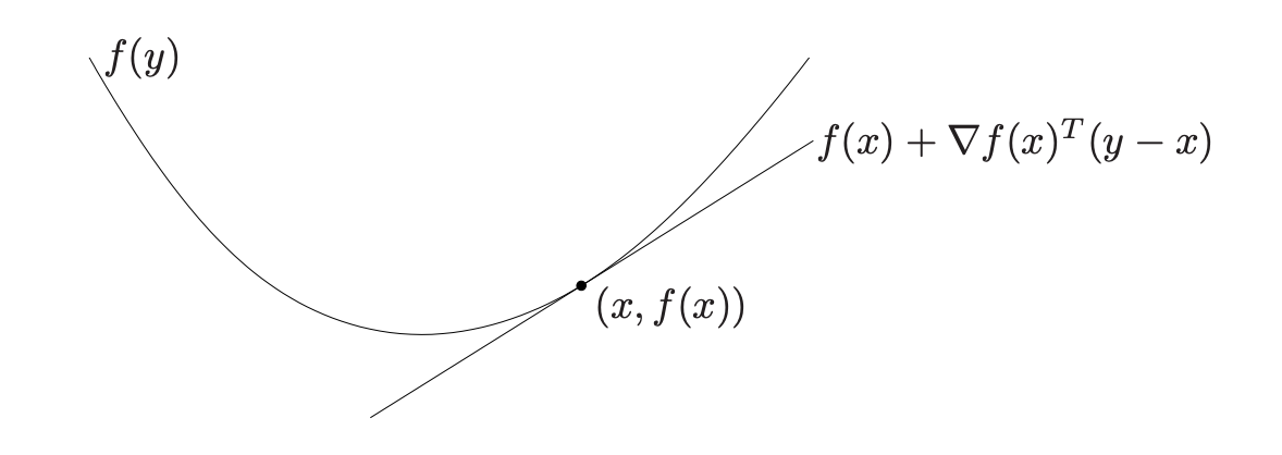
Criterion (1st order condition) Suppose \(f\) is differentiable. Then \(f\) is convex iff \(dom(f)\) is convex and \(\forall x, y \in dom(f)\)
It states that the first taylor approximation is a global underestimator for convex function. Conversely , if the first Taylor approximation is aways a global underestimator, then the function is convex.
Criterion (2nd order condition) Suppose \(f\) is twice differentiable, then \(f\) is convex iff \(dom(f)\) is convex and its Hessian is positive semidefinite \(\forall x \in dom(f)\)
For a function on \(\mathbb{R}\), this reduces to the simple condition \(f''(x) \geq 0\)
quadratic function
Consider the quadratic function \(f: \mathbb{R} \to \mathbb{R}\) given by
with \(P \in S^n\). \(f(x)\) is convex iff \(P \succeq 0\)
Definition (sublevel set, superlevel set) The \(\alpha\)-sublevel set of \(f: R^n \to R\) is defined as
Corollary (sublevel set and convex) Sublevel sets of a convex function are convex. Note that the converse is not true: a function can have all its sublevel sets convex, but not be a convex function. (e.g: \(f(x) = e^{-x}\))
Definition (epigraph) The epigraph of a function \(f: R^n \to R\) is defined as
\(dom(f)\) can be seen as a projection of \(epi(f)\).
Theorem (epigraph and convexity) A function is convex iff its epigraph is a convex set
Many results for convex functions can be proved geometrically by using epigraphs and apply results for convex sets.
convex set and indicator function
A convex set \(X\) can also be mapped to a indicator function \(\delta(x|X)\). A set if convex iff its indicator function is convex
2.2. Closedness and Semicontinuity
Definition (closed function) A function \(f\) is a closed function if its epigraph is a closed set.
Definition (semicontinuous) A function \(f\) is called lower semicontinuous at \(x \in \mathcal{X}\) if
for every sequence \({x_k} \subset \mathcal{X}\) with \(x_k \to x\). We say that \(f\) is lower semicontinuous at each point \(x\) in its domain \(\mathcal{X}\). Upper semicontinuous is defined that \(-f\) is lower semicontinuous.
2.3. Subgradient
Subgradient can be defined wrt non-differentiable function, it always exists.
Definition (subgradient) A subgradient of a convex function \(f\) at \(x\) is any \(g\) such that
Definition (subdifferential) Set of all subgradient is called subdifferential
If \(f\) is differentiable then, \(\partial f(x) = \{ \nabla f(x) \}\)
subdifferential of indicator function
Consider the indicator function \(I_C(x)\)
For \(x \in C\), \(\partial I_C(x) = N_C(x)\) where \(N_C(x)\) is the normal cone at \(x\)
Lemma (calculus of subgradient)
- scaling: \(\partial (\alpha f) = \alpha (\partial f)\)
- addition: \(\partial (f_1 + f_2) = \partial f_1 + \partial f_2\)
- affine: \(\partial g(x) = A^T \partial f(Ax+b)\) where \(g(x)=f(Ax+b)\)
2.4. Operations that preserve convexity
Proposition (nonnegative weighted sum) Nonnegative weight sum of convex function is convex function
Proposition (affine mapping) Affine mapping preserves convexity
least square problem is convex
that least square problem is a convex problem because norm is convex and its inside is an affine function.
Proposition (pointwise maximum) If \(f_1, f_2\) are convex function then their pointwise maximum is also convex
Extending this to infinite set of convex, we have the supremum
Proposition (supremum) If for each \(y\), \(f(x,y)\) is convex in \(x\), then its supreme over \(y\) is also convex
where the domain is
Proposition (scalar composition) Suppose \(f(x) = h(g(x)))\) where \(h: R \to R\) and \(g: R^n \to R\), then the composition rules is
- \(f\) is convex if \(h\) is convex, extended \(h\) is nondecreasing and \(g\) is convex
- \(f\) is convex if \(h\) is convex, extened \(h\) is nonincreasing and \(g\) is concave
Proposition (vector composition) Suppose \(f(x) = h(g_1(x), ..., g_k(x))\) where \(h: R^k \to R, g_i: R^n \to R\). \(f\) is convex if \(h\) is convex and nondecreasing in each argument, \(g\) is convex
Proposition (infimum) If \(f\) is convex in $(x,y) $ and \(C\) is a convex nonempty set, then the function \(g\) is convex if some \(g(x) > -\infty\)
Notice the difference between previous sup and inf: the inf requires \(y\) to be minimized over a convex set where sup does not require anything.
distance to a set
The distance of a point \(x\) to a set \(S\) is defined as
This function is convex
Proposition (perspective of a function) If \(f: R^n \to R\), then the perspective function of \(f\) is the function \(g: R^{n+1} \to R\) defined by
with domain
euclid norm squared
The perspective function on \(f(x)=x^Tx\) is convex
KL divergence
Applying perspective to the convex function \(f(x)=-\log(x)\), we know the convexity of the following
Taking sum, we show the KL divergence is convex over the joint discrete probability distribution \((p,q)=(p_1, ..., p_n, q_1, ..., q_n)\) where \(p=(p_1, ..., p_n), q=(q_1, ..., q_n)\)
2.5. Conjugate function
Definition (conjugate function) Let \(f: R^n \to R\). The function \(f*: R^n \to R\), defined over the dual space as
The domain of conjugate function consists of \(y \in R^n\) for which the sup is bounded.
Conjugate function \(f*\) is a convex function because it is taking sup over a affine function of \(y\). This is true regardless of \(f\)'s convexity.
conjugate of convex quadratic function
The conjugate of \(f(x) = \frac{1}{2}x^TQx\) with \(Q\) positive definite, then
conjugate of indicator function
The conjugate of indicator function f a set \(S\), i.e \(I(x) = 0\) with \(dom(I)=S\) is the support function of \(S\)
conjugate of log-sum-exp
The conjugate of log-sum-exp \(f(x) = \log (\sum_i e^{x_i})\) is the negative entropy function
with the domain restricted to the probability simplex.
Corollary (Fenchel's inequality) from the conjugate definition, it is obvious that
Lemma (conjugate's conjugate) If \(f\) is convex and closed, then
2.6. Quasiconvex functions
Definition (quasiconvex) A function \(R^n \to R\) is called quasiconvex if its domain and all sublevel sets
for all \(\alpha \in R\) are convex. A function is quasiconcave if \(-f\) is quasiconvex. It is quasilinear if it is both quasiconvex and quasiconcave
log is quasilinear
\(\log x\) on \(R_}\) is both quasiconvex and quasiconcave therefore quasilinear.
linear-fractional function is quasilinear
The function
with \(dom f=\{ x | c^Tx+d > 0 \}\) is quasiconvex and quasiconcave (quasilinear)
Criterion (quasiconvex functions on R) A continous function \(R \to R\) is quasiconvex in following cases
- \(f\) is nondecreasing
- \(f\) is nonincreasing
- \(f\) is nonincreasing until a point and nondecreasing after that
Criterion (Jensen's inequality for quasiconvex function) A function \(f\) is quasiconvex iff domain is convex and for all \(x,y\) and \(\theta \in [0, 1]\)
Criterion (first order condition) Suppose \(f: R^n \to R\) is differentiable. Then \(f\) is quasiconvex iff domain is convex and for all \(x,y \in dom(f)\)
Criterion (second order condition) Suppose \(f\) is twice differentiable. If \(f\) is quasiconvex, then for all \(x \in dom(f), y \in R^n\)
2.7. Log-Concave Function
Definition (log-convex) A function \(f\) is log concave iff \(\log f(x)\) is concave: for all \(x,y \in \text{dom} f, \theta \in [0, 1]\), we have
which means the value of average is at least the geometric mean
Notice log-convex and log-concave are not symmetric:
- A log-convex function is convex and is quaiconvex, a log-concave function is quasiconcave, however it is not necessarily a concave function.
- log-convex is preserved under sum, but log-concave is not.
2.8. Convexity wrt generalized inequality
Definition (K-nondecreasing) A function \(f: R^n \to R\) is called \(K\)-nondecreasing if
matrix monotone
- \(tr(X^{-1})\) is matrix decreasing on \(S_{^n\)
- \(\det(X)\) is matrix increasing on \(S_{++}^n\)
Criterion (monotonicity) A differentiable function \(f\), with convex domain, is \(K\)-nondecreasing iff
This is analagous to \(f\) is an nondecreasing function iff \(f'(x) > 0\). Notice the difference here is it requires the dual inequality \(K^*\)
Definition (K-convex) A function \(f: R^n \to R^m\) is called K-convex if for all \(x,y\) and \(\theta \in [0, 1]\)
3. Duality
3.1. Lagrange Dual Function
The main advantage of the Lagrangian dual function is, that it is concave even if the problem is not convex.
Definition (Lagrangian) The Lagrangian \(L: R^n \times R^m \times R^p \to R\) associated with the standard form optimization problem is
\(\lambda\) is called the Lagrange multiplier and \(\nu\) is called dual variables. Domain \(\mathcal{D} = \mathrm{dom} f_i \cap \mathrm{dom} h_i\)
Definition (dual function) The Lagrange dual function is the minimum value over \(x\)
Dual function over \((\lambda, \nu)\) is concave even the original problem is not convex.
Lemma (lower bound property) One of the motivations of Lagrangian is to gives the lower bound on the optimal value of the original problem.
This is because for any feasible point \(x\), we have \(f_i(x) \leq 0, h_i(x)=0\), for any \(\lambda \geq 0\)
Then we know
Taking \(\inf_x\) yields the conclusion of the lower bound.
3.2. Lagrange Dual Problem
Each pair of \((\lambda, \nu)\) gives a lower bound to the primal problem, a natural question is to ask what is the best lower bound \(g(\lambda, \nu)\).
Definition (dual problem) The Lagrange dual problem associated with the primal problem is a convex optimization problem even the primal problem is not
Dual feasible means there exists a pair \((\lambda, \nu)\) such that \(\lambda \succeq 0, g(\lambda, \nu) > -\infty\). We refer to \((\lambda^*, \nu^*)\) as dual optimal if they are optimal for the dual problem
The dual problem is always a convex optimization problem even the primal problem is not convex
dual problem of LP
Consider the standard form of LP
The dual function is when \(A^T\nu - \lambda + c = 0\)
Combined with the constraint \(\lambda \succeq 0\). The dual problem is
Proposition (weak duality) The optimal value of the dual problem, denoted \(d^*\) is by definition, the best lower bound on the optimal value of the primal problem \(p^*\), therefore
This property is called the weak duality
Proposition (strong duality) The strong duality holds when the optimal duality gap is zero
The strong duality does not always hold, one of condition to make it hold is the Slater's condition
Criterion (Slater, Sufficiency) The primal problem is convex optimization (\(f_i(x)\) is convex) and there exists a strictly feasible point (i.e. \(x \in \text{relint}(\mathcal{D})\))
In the case of affine constraint, the inequality needs to be strict. Therefore LP always achieves the strong duality.
Slater's condition also implies that the dual optimal value is attained when \(d^* > -\infty\)
Definition (proof, certificate) If we can find a dual feasible \((\lambda, \nu)\), we establish a lower bound on the optimal value of the primal problem: \(p^* \geq g(\lambda, \nu)\). Then the point provides proof or certificate that \(p^* \geq g(\lambda, \nu)\)
3.3. KKT Condition
See this pdf note
Criterion (Karush-Kuhn-Tucker, KKT) For any optimization problem, the following conditions are called KKT condition:
3.3.1. Necessasity
If strong duality holdes (i.e: \(x^*, \lambda^*, \nu^*\) are the primal and dual solutions with zero duality gap), the KKT is a necessary condition (i.e: \(x^*, \lambda^*, \nu^*\) must satisfy KKT condition).
For example, the strong duality is guaranteed if it satisfies the Slater's condition. Note that primal needs not to be convex, the necessity is guaranteed even for non-convex under the strong duality condition.
This can be proved by
The inequality should be all equality:
- \(f_0(x^*) = g(\lambda^*, \nu^*)\) is guaranteed by the strong duality
- \(\inf_x L(x, \lambda^*, \nu^*) = L(x^*, \lambda^*, \nu^*)\) implies \(x^*\) is a stationary point for \(L(x, \lambda^*, \nu^*)\), therefore, stationary condition should be satisfied
- \(\leq L(x^*, \lambda^*, \nu^*) = f_0(x^*)\) implies the complementary slackness
Additionally, \(x^*, \lambda^*, \nu^*\) are feasible points, so both primal and dual feasibility must be satisfied.
3.3.2. Sufficiency
If the primal problem is convex, then it also provides the sufficiency condition: if there exists \(x^*, \lambda^*, \nu^*\) satisfies KKT, then they are primal and dual optimal.
This can be proved by
The first equality is implied by: \(L(x, \lambda^*, \nu^*)\) is convex over \(x\) when the primal problem is convex and \(\lambda^* \geq 0\)
The second equality is implied by complementary slackness and feasibility condition
4. Reference
[1] Boyd, Stephen, and Lieven Vandenberghe. Convex optimization. Cambridge university press, 2004.
[2] Bertsekas, Dimitri P. Convex optimization theory. Belmont: Athena Scientific, 2009.