0x421 Representations
1. Classical Features
1.1. SIFT
1.2. SURF
1.3. BRIEF
Model (BRIEF, Binary Robust Independent Elementary Features)
2. Semi-supervised Learning
Check this blog
2.1. Data Augmentation
Model (AutoAugment)
Model (RandAugment)
- shows that optimal data augmentation depends on model/dataset size, typically, larger dataset/model should use larger augmentation magnitude
- proposes a small search space (number of transformation, magnitude) where a simple grid search can be applied to find optimal augmentation
2.2. Generative Models
The unlabeled dataset can be considered as missing data in the probability framework, which we can optimize using the EM algorithm where the missed labels are unobservable latent variables \(Y\). We infer its labels through posterior \(p(Y|X; \theta)\)
See this book chapter for one of the application in text classification
the drawbacks of such generative models is it needs to model \(P(X,Y)\), which is more complex than the discriminative model \(P(Y|X)\). More parameters are to be estimated, resulting in uncertainty.
2.3. Discriminative Models
Assumption (cluster assumption, smoothness assumptions) the decision boundary should happen in the low data density area, in my understanding it is something like the following example:
Consider two labeled samples on the straight line, \(o..........x\), it makes sense to get some decision boundary looks like this: \(o.....|.....x\),
but if we have some unlabeled data denoted \(*\) and our entire data is \(o***.......x\), it might be better to get the decision boundary to something like this \(o***...|...x\) as the decision boundary \(o***.|.....x\) has high data density.
Model (entropy regularization) This is based on the cluster assumption.
- the decision boundary should happen in the low data density area (high entropy).
- In other word, each label should clear labels (low entropy). entropy regularization favors such decision boundary by reducing entropy (minimizing overlaps) for unlabeled dataset.
Model (pseudo labeling) pseudo labeling can be explained as entropy regularization by encouraging low entropy by assigning pseudo labels
Model (temporal ensemble) maintains pseudo labeling of unlabeled dataset across time with moving average

Model (mean teacher) ensembling model weights across time with moving average to assign pseudo labels
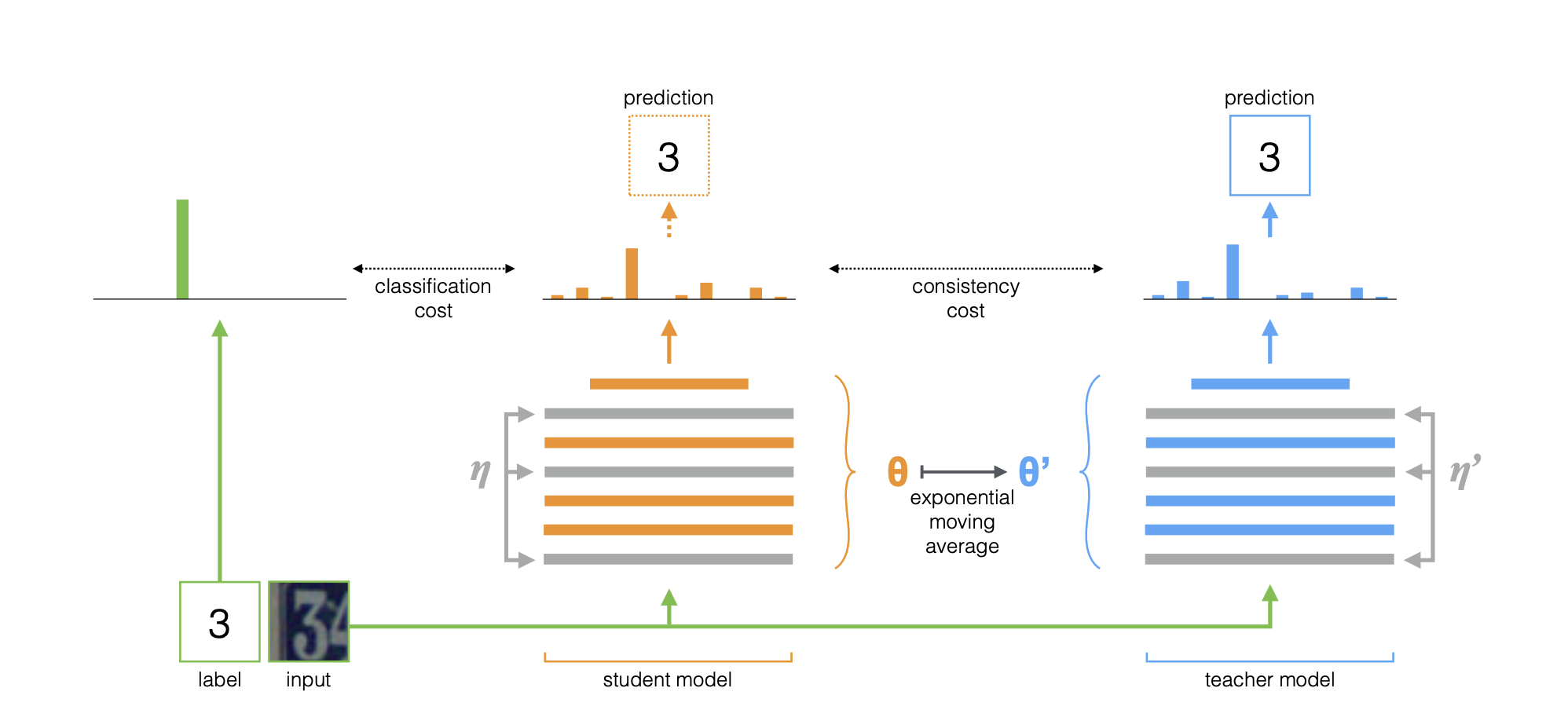
Model (noisy student) the student is larger than teacher and noises are added to student on both model and dataset (not added to teacher)
3. Self-Supervised Learning
This section follows the Cookbook of SSL
3.1. Deep Metric Learning Model
SimCLR/NNCLR/MeanSHIFT/SCL
The deep metric learning family encourages similarity between semantically transformed versions of an image.
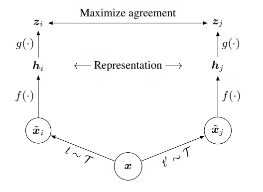
Model (SimCLR) Check illustration of this blog
Learning steps are:
- apply data augmentation (e.g. crop, distortion) to every data point \(x\) in the batch, resulting in positive pair \((\tilde{x}_i, \tilde{x}_j)\)
- use encoder (e.g: ResNet) and pooling (e.g: mean pooling) to encode \(h_i = f(\tilde{x}_i)\)
- project representations \(z_i = g(h_i) = W_2(\text{ReLU}(W_1h_i))\) to do the contrastive loss (\(z_i\) seems to be better than \(h_i\) for contrastive loss)
- apply the contrastive loss
Suppose the minibatch contains \(N\) examples, the augmentation gives \(2N\) data points.the loss function of a positive pair \((i,j)\) is defined as
3.2. Self-Distillation Model
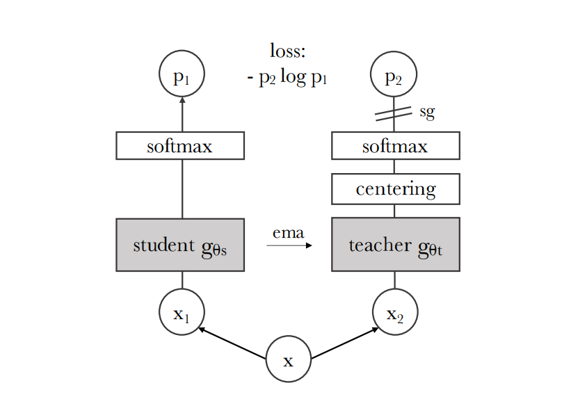
This family feeds two different views to two encoders, and mapping one to the other by means of a predictor.
Model (DINO) self distillation
Model (MoCo v3)
Model (BYOL (bootstrap your own latent))
3.3. Canonical Correlation Analysis Model
3.4. Masked Image Models
3.4.1. Pixel Masked Model
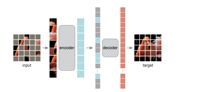
Model (Masked Autoencoder, MAE) The core ideas are
- encoder only operates on the visible subsets of patches
- mask high proportion of images (e.g 75\%)
3.4.2. Token Masked Model
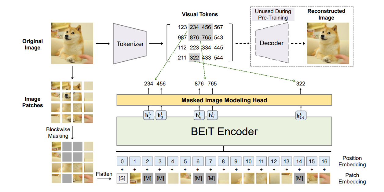
Model (BEiT, Masked Language Model) BERT Pre-Training of Image Transformers
3.4.3. High-level Feature Masked Model
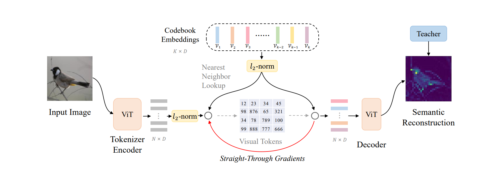
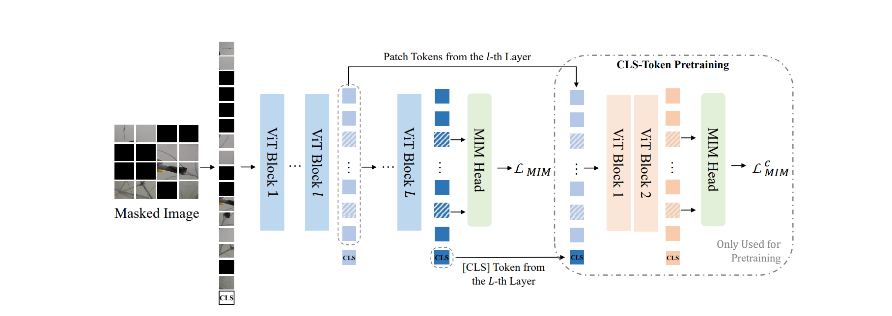
Model (BEiT v2) The core ideas are
- decoder attempts to reconstruct semantic features distilled from teacher models (as shown in the 1st figure)
- a final layer CLS token is concat with intermediate layer's outputs to reconstruct the features (as shown in the 2nd figure). This is to aggregate information to CLS token
3.5. Analysis
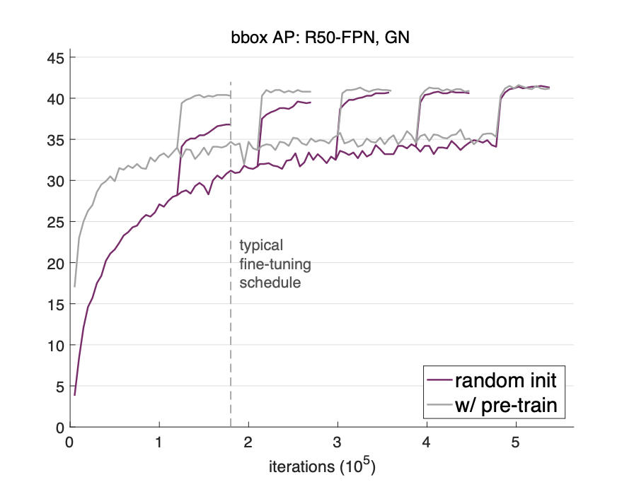
Analysis (rethinking imagenet pretraining) the pretraining does not always help in some cases (Imagenet -> COCO) if we
- train sufficiently longer and good schedule
- with proper normalization
4. Multimodal Feature
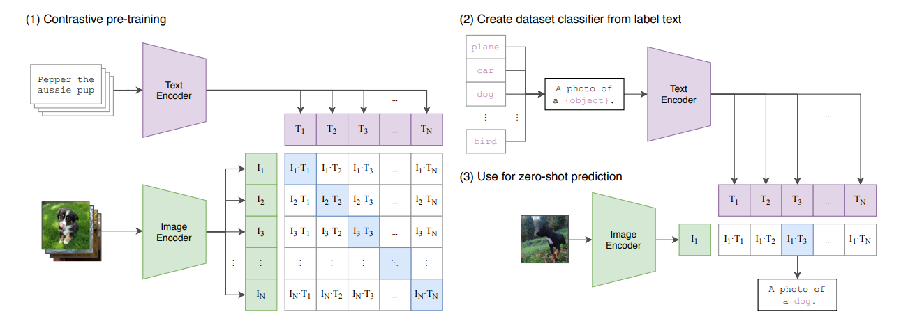
Model (CLIP, Contrastive Language Image Pretraining)
Jointly train a text encoder and image encoder such that the correctly-aligned (text, image) pair has better probability (use cross entropy loss)
This can do a zero-shot prediction using a label text
