0x413 Reinforcement Learning
- 1. Foundation
- 2. Bandit Problem
- 3. MDP
- 4. Basic Algorithms
- 5. Value-based Algorithms
- 6. Policy-based Model
- 7. Reference
1. Foundation
The most important aspect in RL is that it uses training info that evaluates the action taken rather than instructs by giving correct action: it only indicates how good an taken action was, but do not tell whether it was the best or worst. In the instructive setting, the instruction is independent of the action taken.
A lot of machine learning problems are one-shot, in reinforcement learning, we care about sequential decisions: each decision we make have consequences in the future.
RL problems can be expressed as a system consisting an agent and an environment. The system repeats the following circles,
- An environment produces information which describes the state \(s_t\) of the system
- An agent interacts with the environment by observing the state and using this information to select an action \(a_t\).
- The environment accepts the action and transitions into the next state, then return the next state and a reward \(r_t\) to the agent
There are two problems we need to solve
Definition (prediction vs control)
- prediction: evaluate the value function
- control: find the optimal policy
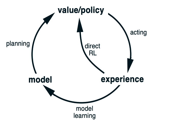
Definition (direct vs indirect RL)
- direct RL: directly improve the value/policy from the real experience
- indirect RL: learn the model first and then use it to do the planning
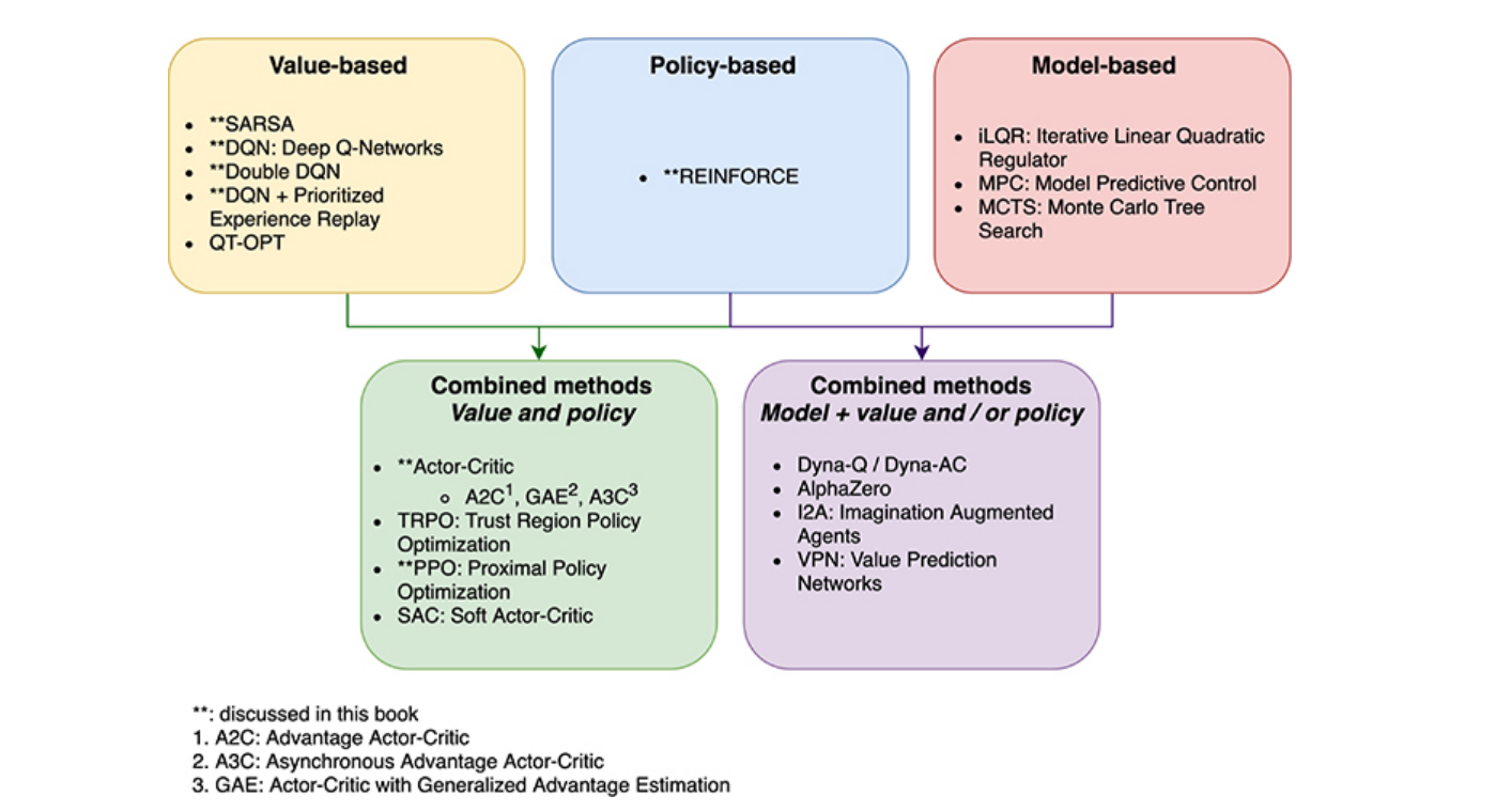
Reinforcement learning can be divided into three categories:
Family (model based algorithms) It learns the model of the environment
Purely model based approaches are commonly applied to games with a target state: winning or lossing in a game. (e.g: MCTS (monte carlo tree search))
Advantage:
- sample efficiency
Disadvantage:
- models are hard to come by
- may learn irrelevant details
Family (value based algorithms) This family learns the value function \(V\) or \(Q\), and use these or generate a policy (e.g: SARSA, DQN)
A policy can be generated from those values (e.g: greedy, SARSA)
Advantage:
- sample efficiency
- low variance
Disadvantage:
- usually limited to discrete actions
- convergence is not guaranteed
Family (policy based algorithms) It learns a good policy \(\pi\), which should generate actions that produce good reward (e.g: REINFORCE)
Advantage:
- very general approach, can be applied to problem with any types of actions (e.g: continuous, discrete)
- directly optimize the objective function
- local convergence
- learn useful stochastic policies (e.g: optimal policy of iterated rock-paper-scissors game is uniform random: Nash equilibrium)
- sometimes policy are simple while models and value are complex
Disadvantage:
- high variance
- sample inefficiency
There are other concepts to distinguish the RL models:
Concept (model-based vs model-free) Whether an algorithm uses a model of an environment’s transition dynamics
By a model of the environment, we mean anything that an agent can use to predict how the environment will respond to its actions
- distribution models: model produce a description of all possibilities and probabilities
- sample model: a distribution model produce an individual possibility
Concept (on-policy vs off-policy) Whether an algorithm learns with data gathered using just the current policy
2. Bandit Problem
2.1. Multi-arm Bandit
Suppose we play a game in \(n\) rounds, at each round \(t\), player chooses an action \(j\) from a finite set of possible choices called arms \(\{ 1, ..., m \}\). A random reward \(X_j(t)\) is drawn from some distribution.
At the end of each turn \(t\), we can estimate the empirical mean reward of arm \(j\) by
where \(T_j(t-1)\) is the total number that \(j\) has been played.
Our goal is to minimize the regret
where \(\mu_j\) is the expected payoff of arm \(j\), and \(\mu_*\) is the expected payoff best arm.
There are many applications for multi-armed bandit, for example NY Times uses it to determine which news to show. It can be considered as an alternative to massive AB testing, to test many alternative options at the same time (instead of doing it pairwise)
Algorithm (\(\epsilon\)-greedy) With probability \(\epsilon_t\), play an arm randomly, otherwise select the "best" arm found so far
There are many works to show the regret bound of this algorithm, it is at most logarithmic in \(n\).
Paper (regret bound, Lai, Robbins 1985) the optimal machine is played exponentially more often than any other machine asymptotically.
For any suboptimal machine \(j\), we have
where \(p_j\) is the reward density for this suboptimal machine.
Paper (regret bound, Auer 2022) shows the optimal logarithmic regret is also achievable uniformly over time.
Algorithm (UCB, upper confidence bound) At each round, chooses the arm with the highest upper confidence interval given by
The regret bound of this also grows logarithmically in \(n\)
Algorithm (Gradient Bandit Algorithm) choose the action based on preference \(H\) instead of value function.
Preference is updated by
depending on \(a = A_t\) or \(a \neq A_t\)
It is a stochastic approximation to gradient ascent
2.2. Contextual Bandit
3. MDP
We assume the the transition to the next state \(s_{t+1}\) only depends on the previous state \(s_{t}\) and action \(a_t\), which is known as the markov property
Definition (Markov Process) Markov Process can be defined as (S, P)
- S: state space
- P: transition prob
Definition (Markov Reward Process) Markov Reward Process \((S, P, R)\)
Definition (Bellman function)
- Each state can be assigned value function.
- the value function can be estimated using Bellman function
- Explicit solution of this Bellman function requires O(n) for inverse matrix operation
- Other methods can be Monte carlo ...
3.1. Markov Decision Process
Definition (Markov Decision Process) Markov Decision Process is defined as a 4-tuple \((\mathcal{S}, \mathcal{A}, \mathcal{R}, P)\)
- \(S\): state space (depend on previous state and action)
- \(A\): action space
- \(R\): reward space
The dynamics of the MDP can be summarized by \(p: \mathcal{S} \times \mathcal{R} \times \mathcal{S} \times \mathcal{A} \to -> [0, 1]\)
This four-arg dynamics function \(p\) can compute many other things:
For example, the transition prob distribution:
The expected reward
The interaction between environment and agent can be expressed in Python as
# Given an env (environment) and an agent

for episode in range(MAX_EPISODE):
    state = env.reset()
    agent.reset()

    for t in range(T):
        action = agent.act(state)
        state, reward = env.step(action)
        agent.update(action, state, reward)

        if env.done():
            break
Definition (reward function) The reward function is defined with respect to an episode \(\tau = (s_0, a_0, r_0), ..., (s_T, a_T, r_T)\) the discount ratio \(\gamma\)
The objective \(J(\pi)\) is the expectations of the returns over many trajectories
A return \(R_t\) of a trajectory is defined as the discounted sum of award from timestamp \(t\) to the end of the trajectory
where both \(G_t, R_t\) are random variables.
POMDP
POMDP (partially observable MDP) is a generalization of MDP, which the agent cannot observe the underlying state. it only observes state partially through sensor, so there are two states:
- observable state: the state observed by the agent
- internal state: the state inside the environment
This is the actual model in the real-world
3.2. Policies and Value Functions
Definition (policy) A policy \(\pi\) is how an agent produces the action in the environment to maximize the objective, it is a distribution over actions given state \(\pi(a|x)\)
Definition (state value Function) The state value function \(v\) evaluates a state under a certain policy, it evaluates how good or bad a state is
Definition (action value function, q) The action value function evaluates a (state, action) pair under a certain policy.
Those functions can be estimated by taking average of randomly sample of actual returns (e.g: Monte Carlo) when there are few states. In the case there are very many states, it is practical to maintain \(v_\pi, q_\pi\) as parametrized functions instead.
Definition (advantage function) advantage function is defined as
Definition (Bellman Equation for MDP)
state value function can be derived from action value function
action value function can be derived from next state value function
Merging those two together, we get
3.3. Optimal Policies and Optimal Value Functions
It is well known that there exists an optimal policy \(\pi^*\)
Definition (Optimal Value Function) the optimal state value function is the maximum value function over all policies
MDP is solved if we know the optimal action value function
It is well known that there exists an optimal policy \(\pi^*\)
Theorem (existence of Optimal Policy) a policy is better than another when its value function on all states should be better than the value function for the other
Definition (Bellman Optimality Equation)
optimal value function are recursively related by the Bellman optimality equations
optimal action function can be expanded in the same manner
Unfolding the action value function
Solution of Bellman Optimality Equation
- nonlinear, no closed form solution in general
- Iterative solution methods
4. Basic Algorithms
4.1. Dynamic Programming (Model-based)
DP solves a known MDP
Optimal substructure
- optimal solution can be decomposed into subproblems
Overlapping subproblems
- Subproblems recur many times
- Solutions can be cached and reused
Dynamic programming assumes full knowledge of MDP
for Prediction:
- Input MDP, and policy and output value function v_pi
for Control: - output: optimal value function v_star and optimal policy
4.1.1. Policy Evaluation (Prediction)
First we consider how to compute the state-value function \(v_\pi\) for an arbitrary policy \(\pi\). This is called policy evaluation, or the prediction problem
If the dynamics \(p\) is completely known, then it can be iteratively solved using Bellman expectation backup
It can be shown the sequnece \(v_k\) converges to the fixed point \(v_\pi\). This algorithm is called iterative policy evaluation
4.1.2. Policy Iteration (Control)
Theorem (policy improvement theorem) Let \(\pi, \pi'\) be any deterministic policies such that if for all \(s\)
then the policy \(\pi'\) must be as good as, or better than \(\pi\):
Using this theorem, we can suggest the following algorithm
Model (policy improvment) Given a policy \(\pi\), Evaluate the policy to get \(v_{\pi}(s)\) Improve the policy to \(\pi'\) by acting greedily with respect to \(v_{\pi}\)
this is called policy improvement
Model (policy iteraion) By repeating policy evaluation and policy improvment, we get the policy iteration algorithm.
This policy iteration always converges to \(\pi_{*}\): when the new greedy policy has the same value function as the old policy
This satisfies the Bellman optimality equation, which indicates \(v_\star = v_{\pi'}\)
4.1.3. Generalized Policy iteration (control)
The generalized policy iteration refers to the idea of letting policy-evaluation and policy-improvment processes interact, independent of the granularity and other details of the two processes.
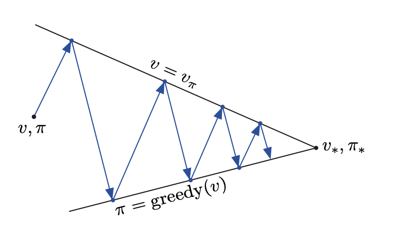
Model (value iteration) We do not need to wait until the value function converge. If we update policy every time updating the value function then it is the value iteration
4.2. Monte Carlo Methods (Model-free)
Unlike the DP, we do not assume complete knowledge of the environment: we only require experience - sample complete episodes from the actual experience.
4.2.1. On-policy Prediction (On-policy)
We assume the model is not available, so we need to estimate action values \(q_\pi(s,a)\) using either of the following:
-
first-visit MC method estimates \(q_\pi(s, a)\) as the average of the returns following first visits to \(s\)
-
every-visit MC method averages the returns following all visits to \(s\)
Note that if a model is available, we still use the state value functions \(v_\pi(s)\)
4.2.2. On-policy Control
We can do similar pilicy iteration in the following manner:
where policy evaluation is done as mentioned in MC Prediction, the policy improvment is done using
To guarantee the convergence, it requires the assumption of the exploring starts
4.2.3. Off-policy Prediction
Off-policy methods are of greater variance and are slower to converge, but they are more powerful and general. It allows the agent to learn from a more diverse set of experiences, which can help it to explore the environment more effectively
There are two policies involved:
- target policy: policy being learned
- behaviror policy: the policy used to generate behavior
We want to estimate \(v_\pi\) or \(q_\pi\) (target policy) but episodes are following another policy \(b\) (behavior policy).
There is a constraint called coverage which says \(\pi(a|s) > 0\) must imply \(b(a | s) > 0\)
Almost all off-policy methods are using importance sampling (my note)
Given a episode \(A_t, S_{t+1}, A_{t+1}, ..., S_T\) and its return \(G_t\), the expectation gives value function of the bahavior policy, not the target policy:
To apply importance sampling, we need to consider the relative probability ratio under two difference policies
Given a episode \(A_t, S_{t+1}, A_{t+1}, ..., S_T\)
Using this ratio, we obtain the value function of target policy
To estimate \(v_\pi(s)\) using previous formula, we can do the ordinary importance sampling
where \(\tau(s)\) is the set of all timestamps in which state \(s\) is visited
or the weighted importance sampling
In the first-visit methods, ordinary importance sampling is unbiased with large variance, weighted importance sampling is biased but with much smaller variance and is strongly preferred. In the every-visit method, both are biased.
4.2.4. Off-policy Control
5. Value-based Algorithms
5.1. Temporal Difference Learning (Model-free)
Recall Monte Carlo do the following prediction
where \(G_t\) is the actual return following time \(t\). It means we must wait until the end of the episode to determine the increment to \(V(S_t)\)
In contrast, TD methods use cached value instead of the waiting complete actual return. For example,
Model (TD(0)) it updates value \(V(S_t)\) toward estimated return \(R_{t+1} + \gamma V(S_{t+1})\)
Because it bases its update in part on an existing estimate, it is called bootstrapping method.
The comparison between MC (left) and TD (right) can be illustrated as following
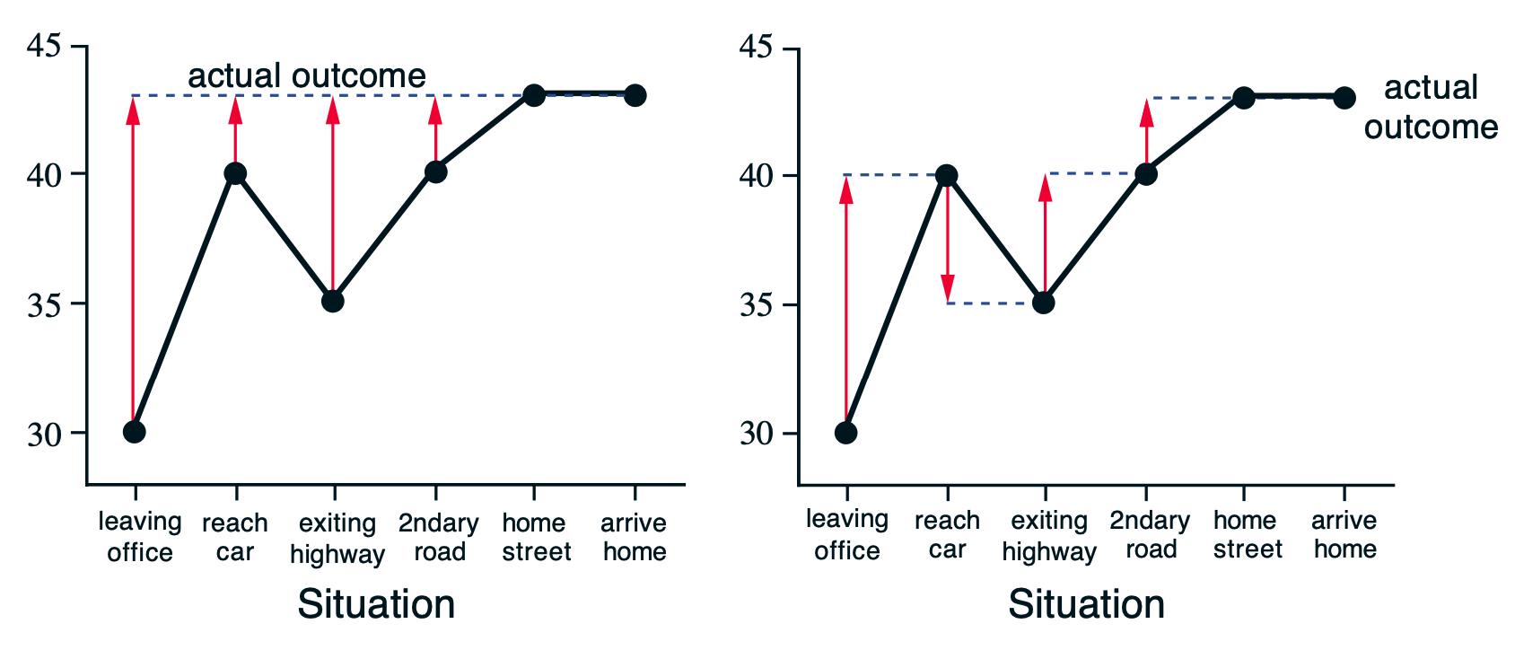 (Reference: from RL Book 2nd version)
It has some bias, low variance (because only one random action in case of TD(0))
It can be generalize to look n steps into the future, we can average multiple n steps
Definition (TD(lambda)) TD(lambda) combines all n-steps return with decaying weight.
5.2. SARSA: On-policy TD Control
Instead of using TD to update state values, we use TD to update action values with a tuple \((S_t, A_t, R_{t+1}, S_{t+1}, A_{t+1})\)
5.3. Q-Learning: Off-policy TD Control
Q-learning learned the action value function \(Q\) to directly approximate \(q_*\) as follows:
It is an off-policy as the next action is obtained by maximizing \(q\) instead of following current policy
6. Policy-based Model
In policy-based algoirhtms, we aim to optimize the policy directly without using a value function
6.1. REINFORCE
The key idea is: during learning, actions that result in good outcomes should become more probable. These actions are positively reinforced. Actions are changed by following the policy gradient.
The policy gradient algorithm solves the following optimization problem
The policy parameter \(\theta\) is updated by gradient ascent
where the policy gradient \(\nabla J\) is defined as
The 2nd equation is done by the score function trick
Intuitively, if the return \(R_t(\tau) > 0\), then the probability of the action \(\pi_\theta(a_t | s_t)\) is increased, otherwise it is decreased
In practice, we approximate this policy gradient with Monte Carlo Sampling
The REINFORCE algorithm is as follows:
1: Initialize learning rate α

2: Initialize weights θ of a policy network πθ

3: for episode = 0, . . . , MAX_EPISODE do

4:       Sample a trajectory τ = s0, a0, r0, . . . , sT, aT, rT

5:       Set ∇θJ(πθ) = 0

6:       for t = 0, . . . , T do

7:            Rt(τ)=Σ^T_{t'=t} γ^{t'−t}*r′t
8:            ∇θ J(πθ) = ∇θJ(πθ) + Rt(τ) ∇θ log πθ(at | st)

9:       end for

10:       θ = θ + α∇θ J(πθ)

11: end for
To reduce the variance of the REINFORCE, one approach is to normalize the reward as
where \(b(s_t)\) might be the value function \(V\), this is related to the Actor-Critic algorithm. Another option is to use the mean over the trajectory
the function which is the discounted rewards minus a baseline is called the advantage function
6.2. Actor-Critic
The REINFORCE algorithm suffers the variance in the gradient estimation, which requires large samples to train. To improve this
we combine the value and policy Based models in Actor-Critic Method
- an actor is a policy-based method, it controls how our agent behaves \(\pi_\theta(s)\)
- a critic is a value-based method, it measures how good the taken action is, \(\hat{q}_w(s, a)\)
Convergence
There are several words dealing global convergence of policy gradient methods:
7. Reference
[0] RL book 2nd
[1] David Silver's reinforcement learning lecture
[2] CMU 10703 Deep Reinforcement Learning and Control
[3] Foundations of Deep Reinforcement Learning: Theory and Practice in Python