0x441 Representations

• 1. Classifical Features
  • 1.1. Acoustic Features
  • 2.1. Linguistic Features
  • 2.2. Phoneme Feature
  • 3. Speaker Features
• Semi-Supervised Learning
  • Data Augmentation
  • Pseudo Labeling
• 4. Self-Supervised Learning
  • 4.1. Nonparametric Bayesian Models
  • 4.2. Autoregressive Models
  • 4.3. Generative Model
  • 4.4. Masked Model
  • 1.2. Neural Codec
  • 4.5. Analysis
  • 4.6. Downstream Tasks
• 5. Multimodal Features
  • 5.1. Speech-Text joint features

1. Classifical Features

1.1. Acoustic Features

Depending on the model, we might use different features. In the traditional models, one example feature set is

• 40 and 60 parameters per frame to represent the spectral envelope
• value of F0
• 5 parameters to describe the spectral envelope of the aperiodic excitation

Feature (GeMAPS, Geneva Minimalistic Acoustic Parameter Set)

This works suggests a minimal set of acoustic descriptor as follows (extracted from the paper)

Frequency related parameters:

• Pitch, logarithmic F0 on a semitone frequency scale, starting at 27.5 Hz (semitone 0).
• Jitter, deviations in individual consecutive F0 period lengths.
• Formant 1, 2, and 3 frequency, centre frequency of first, second, and third formant
• Formant 1, bandwidth of first formant

Energy/Amplitude related parameters:

• Shimmer, difference of the peak amplitudes of consecutive F0 periods.
• Loudness, estimate of perceived signal intensity from an auditory spectrum.
• Harmonics-to-Noise Ratio (HNR), relation of energy in harmonic components to energy in noiselike components.

Spectral (balance) parameters

• Alpha Ratio, ratio of the summed energy from 50–1000 Hz and 1–5 kHz
• Hammarberg Index, ratio of the strongest energy peak in the 0–2 kHz region to the strongest peak in the 2–5 kHz region.
• Spectral Slope 0–500 Hz and 500–1500 Hz, linear regression slope of the logarithmic power spectrum within the two given bands.
• Formant 1, 2, and 3 relative energy, as well as the ratio of the energy of the spectral harmonic peak at the first, second, third formant’s centre frequency to the energy of the spectral peak at F0.
• Harmonic difference H1–H2, ratio of energy of the first F0 harmonic (H1) to the energy of the second F0 harmonic (H2).
• Harmonic difference H1–A3, ratio of energy of the first F0 harmonic (H1) to the energy of the highest harmonic in the third formant range (A3).

2.1. Linguistic Features

In neural TTS, the linguistic feature is just grapheme, subword or words, but in traditional TTS, we are using more detailed linguistic features.

The input \(w\) is usually transformed into linguistic features or linguistic specification. This could be as simple as a phoneme sequence, but for better results it will need to include supra-segmental information such as the prosody pattern of the speech to be produced. In other words, the linguistic specification comprises whatever factors might affect the acoustic realisation of the speech sounds making up the utterance.

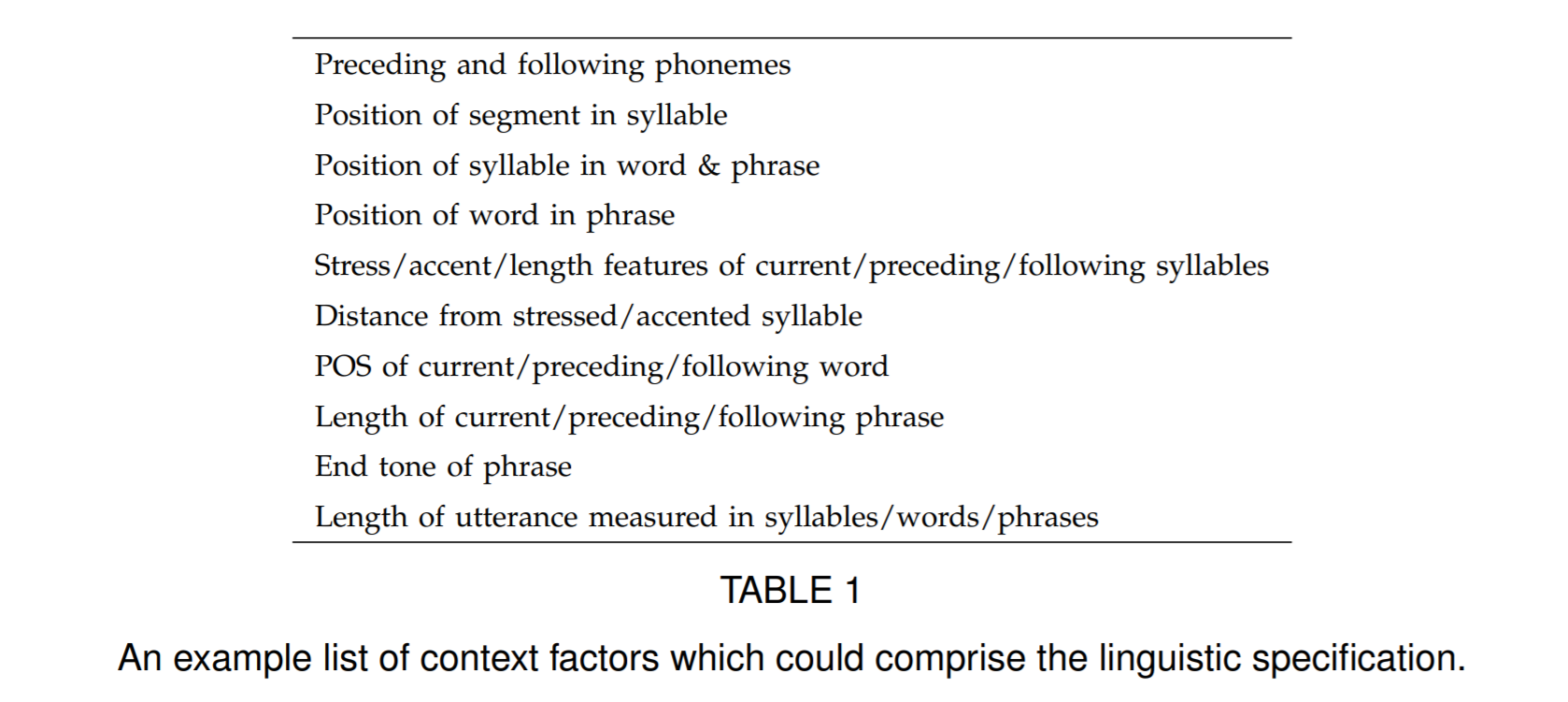
For example, in HTS, the lab file might contain those features

2.2. Phoneme Feature

Phoneme-based TTS models may suffer from the ambiguity of the representation, such as prosody on homophones.

Consider the sentence: To cancel the payment, press one; or to continue, two.

The last word two can be confused with too, whose phoneme sequence is same but prosody is different. (pronunced with pause or not)

Listen to the first samples for difference here

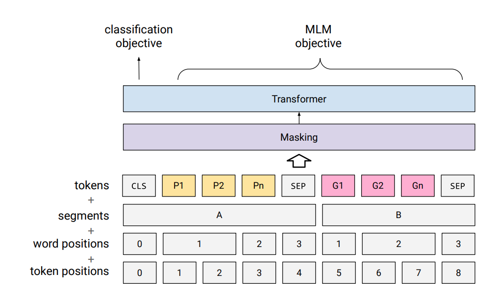
Model (PnG BERT) This work pretrain a BERT-like model by concating phoneme seq and grapheme seq on a large text corpus. Hidden states of phoneme token can be used as input to TTS model.

This concat helps the phoneme to carry info from grapheme and disambiguiate prosody

Model (G2P, 1-1 approach) 1-to-1 approach:

• Issues in Building General Letter to Sound Rules

Model (G2P, N-to-N approach)

Applying Many-to-Many Alignments and Hidden Markov Models to Letter-to-Phoneme Conversion (Github)

• run forward-backword to get the alignment
• segment word into a sequence of letter chunks (by training a different model), then run the aligned models on it.

For a general unicode-based G2P tool, the options are

• unitran: a mapping table can be found here

3. Speaker Features

i-vector, x-vector, d-vector

Semi-Supervised Learning

Data Augmentation

Pseudo Labeling

Model (noisy student)

• use specaugment to add noise
• shallow fusion with a language model

4. Self-Supervised Learning

Here is a self-supervised learning review for speech

4.1. Nonparametric Bayesian Models

Classical Acoustic Unit Discovery using Dirichlet process mixture model

Model (Gibbs sampling) each mixture is a HMM to model subword unit and to generate observed segments of that unit

Gibbs sampling is used to approximate posterior distribution

Model (Variational Inference) Use VI instead of Gibbs Sampling

4.2. Autoregressive Models

Model (CPC, Contrastive Predictive Coding) see the representation note

Model (CPC + Data Augmentation) Applying augmentation in the past is efficient

• pitch modification
• additive noise
• reverberation

Model (APC, Autoregressive Predictive Coding) use RNN to predict frame feature \(n\)-step ahead

• \(n=3\) performs best on phone classification task

4.3. Generative Model

Model (convolutional VAE) convolutional VAE, it proposes an interesting approach to modify speech attributes by shifting VAE's posterior (section 4.2)

Model (hierarchical VAE)

Model (VQ-VAE) compare three different autoencoder approaches: VQ-VAE, VAE, dimension reduction

The conclusion is among the three bottlenecks evaluated, VQ-VAE discards the most speaker-related information at the bottleneck, while preserving the most phonetic information

4.4. Masked Model

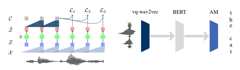
Model (vq-wav2vec)

• First train a quantization model using future prediction task.
• Then use those tokens to pretrain a BERT model

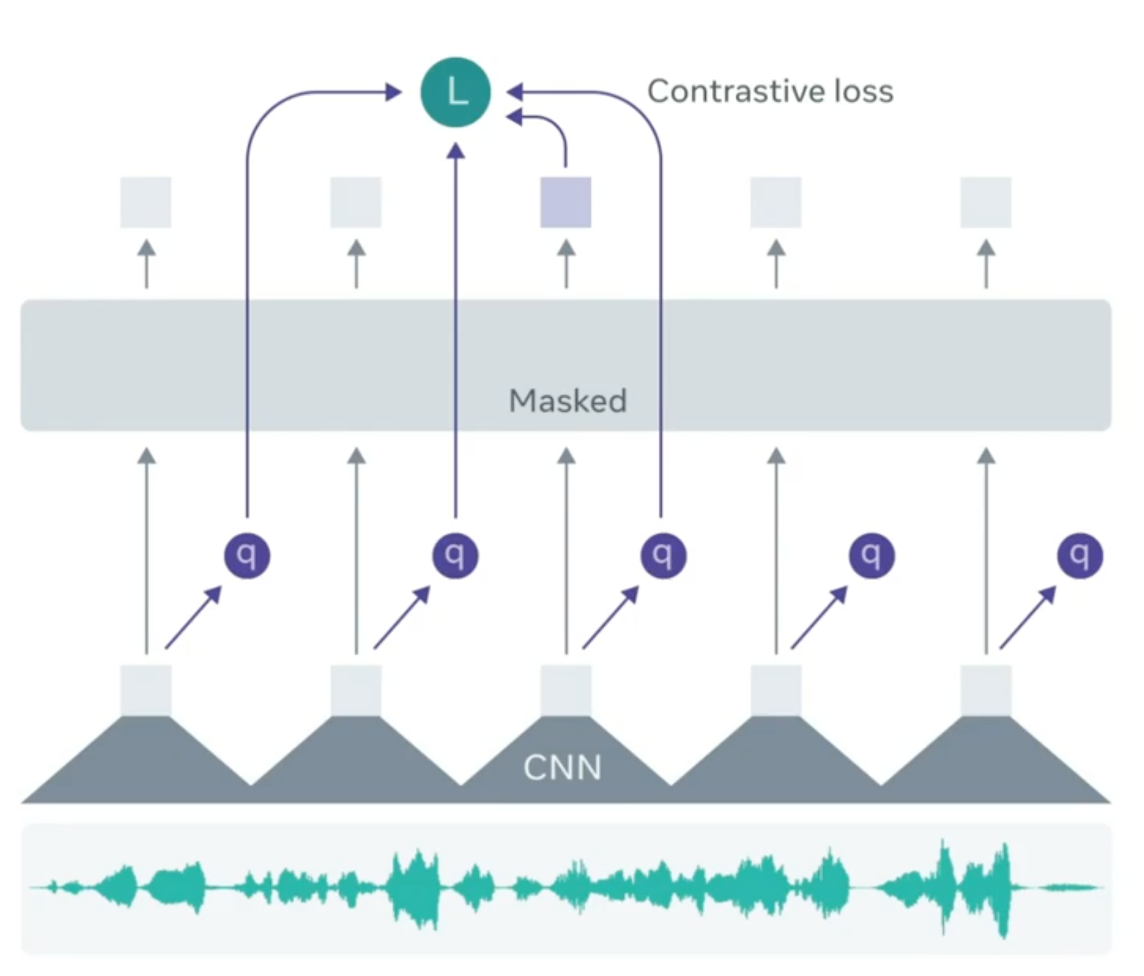
Model (wav2vec2)

Architecture

• Step 1 (local representation): The model first has a feature encoder which takes raw audio into latent speech representation \(f: X \to Z\), producing \(z_1, ..., z_T\). The feature encoder is multi-convolutional encoder, the features \(z_i\) are local features

• Step 2 (contextualized representation): Transformer build contextualized representation \(c_1, ..., c_n\), captures broader global information.

• Step 3 (quantization): local representation \(z_1, ..., z_T\) is quantized to \(q\) using product quantization.

Masking

• sample a certain proportion (0.065) of all time steps to be starting index, and mask consecutive steps (10 step).

Objective

Loss (contrastive loss) masked context representation \(c_t\) should resemble to the quantized \(q_t\) other than the \(K\) distractors.

\[\mathcal{L} = - \log \frac{\exp(sim(c_t, q_t))}{\sum_{q \sim Q} \exp(sim(c_t, q))}\]

where \(Q\) contains the target \(q_t\) and \(K\) distractors.

Loss (diversity loss) max entropy

Fine-tuning

• add a randomalized linear layer to project context feature into the vocabulary

Reference: facebook blog

Model (XLSR) Extending wav2vec2 to multilingual settings.

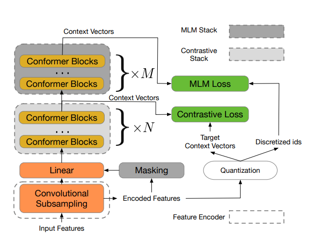
Model (w2v-BERT)

Similar to wav2vec2, but w2v-BERT has both contrastive loss and MLM loss (cross entropy for masked prediction)

The idea of w2v-BERT is to use

• first the contrastive task defined in wav2vec 2.0 to obtain an inventory of a finite set of discriminative, discretized speech units
• then use them as target in a masked prediction task in a way that is similar to masked language modeling (MLM) proposed in BERT for learning contextualized speech representations

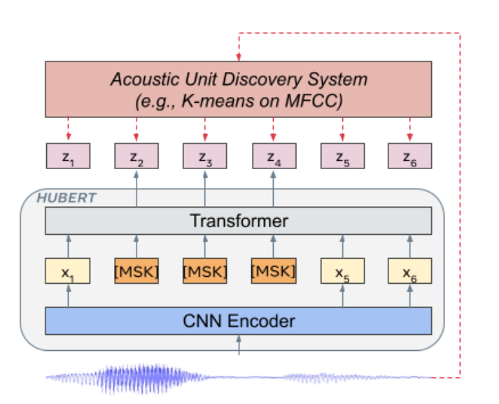
Model (HuBERT, Hidden-Unit BERT)

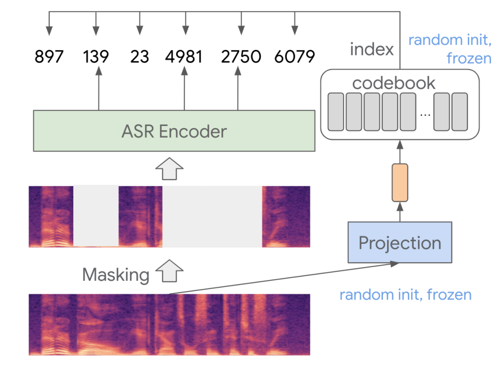
Model (BEST-RQ)

BERT-based Speech pre-Training with Random-projection Quantizer

Model (denoising model, WavLM) combine the masked speech prediction and denoising in pretraining

• inputs are simulated noisy/overlapped speech with masks
• target is to predict the pseudo-label of the original speech on the masked region like HuBERT

1.2. Neural Codec

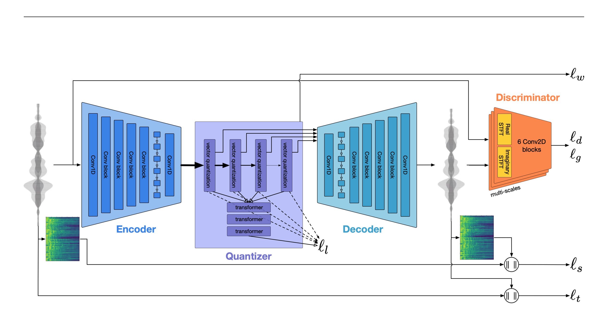
Model (soundstream) encoder-decoder codec model

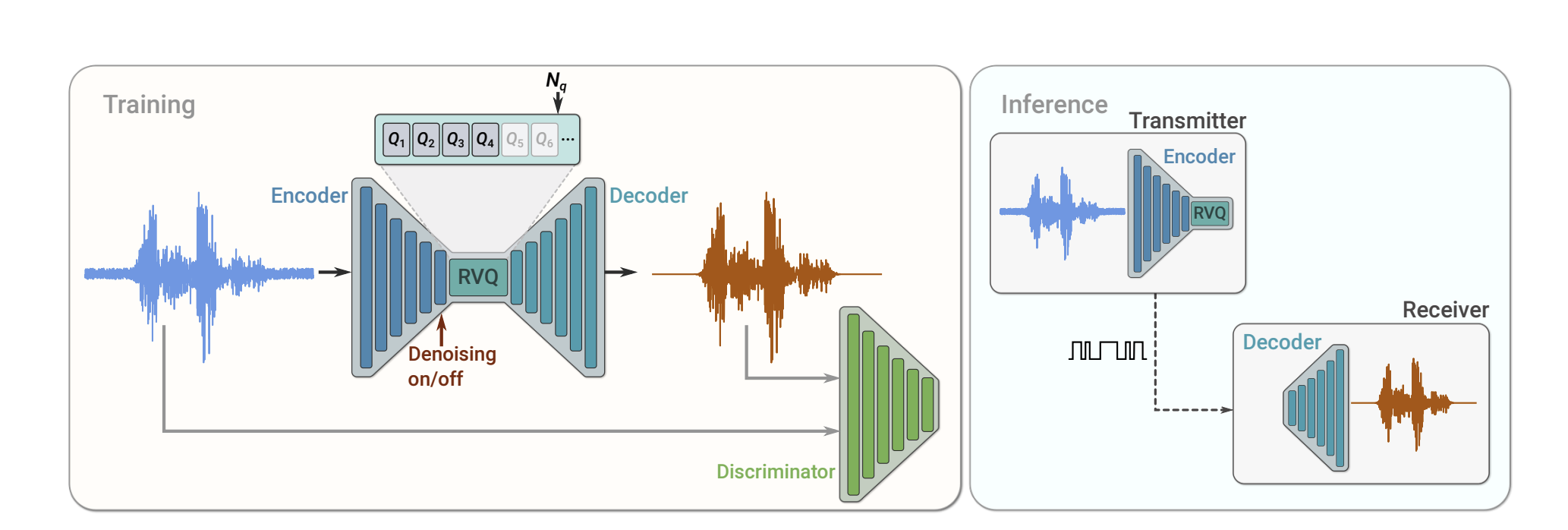
Model (encodec)

4.5. Analysis

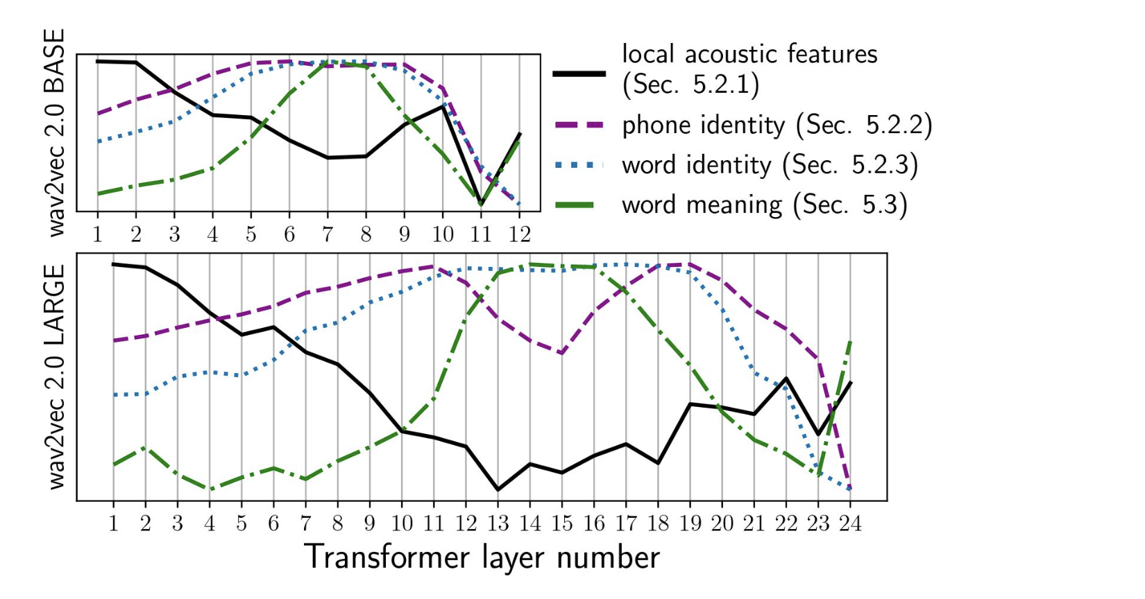
Anaylsis (lingustic information) this work and this work analyzes linguistic information encoded in different layers in wav2vec2

Analysis (discrete vs continuous) Discretized bottleneck seems to be important to learn a good spoken language modeling

Metric (Minimal-Pair ABX, phonetic level) A (/aba/) and B (/apa/) are token representation of the same speaker, X (/aba/) is the representation from (maybe) another speaker, A and X should be more similar than X and B.

The similarity or distance can be computed, for example, using frame-wise angle along the DTW path

This was used in ZeroResource Speech Challenges (e.g: 2020)

Metric (spot-the-word, lexical) Given a pair of words clip (e.g, brick and blick), the model need to classifies which is a real word

4.6. Downstream Tasks

Model (speaker verification and language identification) using wav2vec2

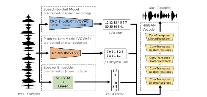
Model (resynthesis)

5. Multimodal Features

5.1. Speech-Text joint features

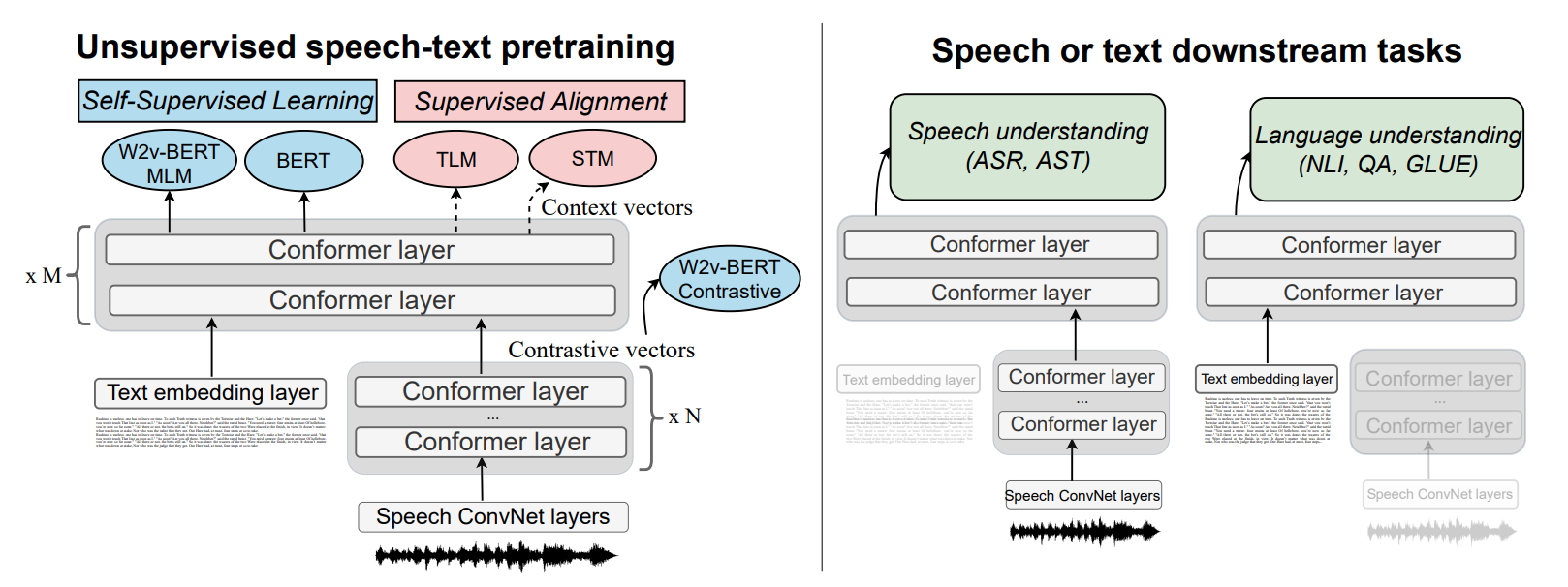
Model (SLAM)

Pretraining objectives

• self-supervised objectives: BERT + w2v-BERT
• alignment loss:
  • translation language modeling: concat speech + transcript to predict masked text or speech
  • speech-text matching: whether text/speech is matched