0x402 Bayesian Inference

1. Movitaion
2. Prior
3. Inference
4. Sampling Methods
5. Approximate Methods
6. Reference

This note follows the Jordan's stats 260 notes and a few chapters from PRML

1. Movitaion

Definition (infinite exchangeability) a sequence of random variable $(x_1, x_2, ...)$ is said to be infiinitely exchangeable if for any $n$, the joint distribution p(x_1, x_2, ..., x_n)$ is invariant to the permutation of indices

\[p(x_1, x_2, ..., x_n) = p(x_{\pi_1}, x_{\pi_2}, ..., x_{\pi_n})\]

infinite exchangeability is related to iid, it is a broader concept, iid implies infinite exchangebility, but not vice versa.

A characterization of infinite exchangeability is given by De Finetti

Theorem (De Finetti) A sequence of random variable is infinite exchangeable iff for all $n$

\[p(x_1, ..., x_n) = \int \prod_1^n p(x_i | \theta)P(d\theta)\]

for some measure $P$ on $\theta$

It says that if we have exchangeable data,

there must exist a likelihood $p(x | \theta)$
there must exist a distribution $P$ on $\theta$
it render the data $x_1, ..., x_n$ conditionally independent

This gives the motivation of the existence of underlying parameter and prior

2. Prior

2.1. Discrete Conjugate Model

2.1.1. Beta-Binomial Model

Suppose we want to model a binary random variable $X \in \{ 0, 1 \}$ with Bernoulli distribution

Given the sample $\mathcal{D}=\{X_1, ..., X_n \}$, we know the likelihood can be written as

\[p(\mathcal{D}|\mu) = \prod_n \mu^{X_n}(1-\mu)^{1-X_n}\]

The ML estimator is

\[\hat{\mu}_{ML} = \frac{m}{N}\]

where $m = \sum_n X_i$ is the sufficient statistics.

The conjugate of Bernoulli/Binomial distribution is the Beta distribution, recall its pdf form is

\[B(\mu | a,b) = \frac{\Gamma(a+b)}{\Gamma(a)\Gamma(b)} \mu^{a-1}(1-\mu)^{b-1}\]

It has the same shape of $\mu^X (1-\mu)^{1-X}$, therefore can serve as the prior and posterior.

The posterior has the form

\[\mu(\mu | m, l, a, b) \propto \mu^{m+a-1}(1-\mu)^{l+b-1}\]

Using the properties of beta distributions, we know the MAP estimator is

\[\hat{\mu}_{MAP} = \frac{m+a-1}{N+a+b-2}\]

however, be careful that posterior mean is different

\[\bar{\mu} = \frac{m+a}{N+a+b}\]

If our goal is to predict the outcome of the next trial, we can

\[p(x=1 | \mathcal{D}) = \int_0^1 p(x=1|\mu)p(\mu|\mathcal{D}) d\mu = E[\mu | \mathcal{D}] = \bar{\mu}\]

2.1.2. Dirichlet-Multinomial Model

2.2. Gaussian Conjugate Model

Jordan's lecture 5 has a good summary

2.2.1. Gaussian Formula

Some useful formula

Lemma (bivariate Gaussian conditional) Assume $(a, b)$ has a bivariate Guassian distribution, then $a | b$ is Guassian with

\[a | b \sim N( \mu_{a | b}, \sigma^2_{a | b})\]

where

\[\mu_{a | b} = \mu_a + \frac{Cov(a, b)}{Var(b)}(b - \mu_b)\]

\[\sigma^2_{a | b} = \sigma^2_a - \frac{(Cov(a, b))^2}{\sigma^2_b}\]

An alternative way to represent them is use $\rho = \frac{Cov(a, b)}{\sigma_{a}\sigma_{b}}$

\[\mu_{a | b} = \mu_a + \rho(\sigma_{a}/\sigma_{b})(b - \mu_b)\]

\[\sigma^2_{a | b} = \sigma_{a}^2 (1 - \rho^2)\]

Lemma (multivariate Gaussian conditional)

Given a joint Gaussian distribution $N(x|\mu, \Sigma)$ with the precision matrix $\Lambda = \Sigma^{-1}$

and $x = (x_a, x_b)$

\[\mu = (\mu_a, \mu_b)\]

\[\Sigma = \begin{pmatrix} \Sigma_{aa} & \Sigma_{ab} \\ \Sigma_{ba} & \Sigma_{bb} \\ \end{pmatrix} \Lambda = \begin{pmatrix} \Lambda_{aa} & \Lambda_{ab} \\ \Lambda_{ba} & \Lambda_{bb} \\ \end{pmatrix}\]

The conditional distribution is given by

\[p(x_a | x_b) = N(x|\mu_{a|b}, \Sigma_{a|b})\]

where

\[\mu_{a|b} = \mu_a + \Sigma_{ab}\Sigma_{bb}^{-1}(x_b - \mu_b)\]

\[\Sigma_{a|b} = \Sigma_{aa} - \Sigma_{ab}\Sigma_{bb}^{-1}\Sigma_{ba}\]

An alternative way to represent them is to use precision matrix where

\[\mu_{a|b} = \mu_a - \Lambda_{aa}^{-1}\Lambda_{ab}(x_b - \mu_b)\]

\[\Sigma_{a|b} = \Lambda_{aa}^{-1}\]

Lemma (linear Gaussian conditional)

Suppose we have two random variables, $x, y$ whose distributions are given as

\[p(x) = N(x | \mu_x, \Sigma_x)\]

\[p(y|x) = N(y | Ax+b, \Sigma_y)\]

This is an example of a linear Gaussian system,

The joint distribution $z=(x,y)$ is

\[p(z) = N(\mu_z, \Sigma_z)\]

where

\[\mu_z = (\mu_x, A\mu_x + b)\]

\[Cov(z) = \begin{pmatrix} \Sigma_x & \Sigma_x A^T \\ A \Sigma_x & \Sigma_y + A \Sigma_x A^T \end{pmatrix}\]

the marginal distribution of $y$ is given by

\[p(y) = N(y|A\mu_x + b, \Sigma_y + A\Sigma_x A^T)\]

the posterior is given by

\[p(x|y) = N(x| \mu_{x|y}, \Sigma_{x|y})\]

where

\[\Sigma_{x|y}^{-1}=\Sigma_x^{-1} + A^T \Sigma_y^{-1}A\]

\[\mu_{x|y} = \Sigma_{x|y} [ A^T \Sigma_y^{-1} (y-b) + \Sigma_x^{-1}\mu_x]\]

2.2.2. Random Mean, Fixed Variance

Lemma Conjugate distribution of $\mu$ is normal distribution. Suppose the prior distribution of $\mu$ is $\mathcal{N}(\mu_0, \sigma^2_0)$, then the posterior distribution is

\[p(\mu | x) = \mathcal{N}(\mu_N, \sigma^2_N)\]

where

\[\mu_N = \frac{\sigma^2}{N\sigma^2_0 + \sigma^2} \mu_0 + \frac{N \sigma^2_0}{N\sigma^2_0 + \sigma^2} \mu_{ML}\]

\[\frac{1}{\sigma^2_N} = \frac{1}{\sigma^2_0} + \frac{N}{\sigma^2}\]

2.2.3. Fixed Mean, Random Variance

Lemma (Posterior) Conjugate distribution of precision $\lambda$ is Gamma distribution. Suppose the prior distribution is Gamma distribution with $(a,b)$ hyperparameter, then posterior Gamma distribution is

\[a_N = a_0 + \frac{N}{2}\]

\[b_N = b_0 + \frac{N}{2}\sigma^2_{ML}\]

Lemma (prediction, marginalization)

We might want to compute the probability of some new data given old data,

\[p(x_{new} | x, \mu, a, b) = \int p(x_{new} | x, \mu, \tau, \alpha, \beta)p(\tau | x, \alpha, \beta) d\tau\]

This integral can be reduced to the student's t-distribution

\[p(x | \mu, a, b) = \int N(x | \mu, \tau^{-1}) G(\tau | a, b) d\tau = \frac{\Gamma(a+1/2)b^a}{\Gamma(a)}(\frac{1}{2\pi})^{1/2}[b+\frac{(x-\mu)^2}{2}]^{-a-1/2}\]

where $\mu=2a, \lambda=a/b$

2.2.4. Random Mean Random Variance

The multivariate version is the Wishart distribution

Conjugate distribution of $\sigma$ is inverse-Gamma distribution

Conjugate distribution of both mean and precision is called normal gamma distribution

2.3. Uninformative Prior

objective Bayesians instead prefer priors which do not strongly influence the posterior distribution. Such a prior is called an uninformative prior

2.3.1. Jeffrey Prior

Definition (Jeffery prior) Jeffery prior is motivated to be invariant of variable transformation, it is defined as

\[\pi_J(\theta) \propto I(\theta)^{1/2}\]

where $I$ is the Fisher information,

\[I(\theta) = - E_\theta [\frac{d^2 \log p(X | \theta) }{d\theta^2}]\]

It can be shown using chain rules:

\[I(\phi) = -E[\frac{d^2 \log p(X | \phi) }{d\phi^2}] = -E[\frac{d^2 \log p(X | \theta) }{d\theta^2}](\frac{d\theta}{d\phi})^2 + E[\frac{d \log p(X|\theta)}{d\theta}] \frac{d^2 \theta}{d\phi^2}\]

Using the expectation of score function, we get

\[I(\phi) = I(\theta)(\frac{d\theta}{d\phi})^2\]

2.3.2. Reference Prior

3. Inference

3.1. Estimation

3.1.1. Bayes Estimator

Definition (Bayes risk) In Bayesian analysis we would use the prior distribution $\pi(\theta)$ to compute an average risk, known as the Bayes risk

\[R_{B} (\delta) = \int_{\Theta} R(\theta, \delta) \pi(\theta) d\theta\]

The Bayes estimator or Bayes decision rule is one which minimizes the expected risk:

\[\delta_{B} = \text{argmin}_{\delta} (R_B(\delta))\]

An alternative approach is to use minimax risk

The Bayes risk can be rewritten using posterior risk $r(\delta | x^n)$ where

\[r(\delta | x^n) = \int L(\theta, \delta) \pi(\theta | x^n) d\theta\]

Theorem (Bayes estimator) The Bayes risk satisfies

\[R_B(\delta) = \int r(\delta | x^n) m(x^n) dx\]

where the Bayes estimator is to minimize posterior risk for each $x$

\[\delta_B = \text{argmin}_\delta r(\delta | x^n)\]

Bayes estimator for mean square error

For squared error loss, the posterioir risk is

\[r(\delta | x^n) \int_\theta (\theta - \delta)^2 \pi(\theta | x) d\theta = E((\delta - \theta)^2 | x)\]

The minimizer is the Bayes estimator, it is known as the minimum mean square error (MMSE) estimator

\[\delta_B = E[\theta | x]\]

Bayes estimator for other losses

If $L(\theta, \delta) = | \theta - \delta|$, then the Bayes estimator is the median of posterior, if loss is 0-1 loss, then the Bayes estimator is the mode of posterior

3.1.2. EM algorithm

The goal of the EM algorithm is to find MLE or MAP for models having latent variables or randomly missing values.

The set of observed data is $X$, the latent variables are $Z$, the log likelihood function (evidence) is given by

\[\log p(X | \theta) = \log (\sum_Z p(X, Z | \theta))\]

where the summation over latent variables inside the logrithm (they are typically some mixture models). therefore intractable. To maximize wrt $\theta$, we apply the ELBO decomposition

\[\log p(X | \theta) = \text{ELBO} + KL(q(Z) || p(Z|X))\]

we repeat the following procedures optimizing two terms on the right hand:

expectation step evaluate posterior $p(Z | X, \theta^{old})$ and set

\[q(Z) := p(Z | X, \theta^{old})\]

This is to optimize the 2^nd KL term on the right side. The left side remains same as it does not depend on $q$, therefore ELBO get maximized.

maximization step evaluate new $\theta^{new}$ wrt ELBO

\[\theta^{new} = \text{argmax}_\theta E_{q(Z)} \log [\frac{p(X,Z; \theta)}{q(Z)}]\]

This is equivalent to maximize the following $\mathcal{Q}$ function as denominator $q(Z)$ is fixed and does not depend on $\theta^{new}$

\[\theta^{new} = \text{argmax}_\theta \mathcal{Q}(\theta, \theta^{old})\]

where

\[\mathcal{Q}(\theta, \theta^{old}) = E_{Z \sim p(Z | X, \theta^{old})} [\log p(X,Z | \theta)]\]

3.2. Hypothesis Testing

3.2.1. Model Comparison

Suppose we want to compare a set of models $\{ \mathcal{M}_i \}$, we wish to evaluate the posterior

\[p(\mathcal{M}_i | \mathcal{D}) \sim p(\mathcal{M}_i) p(\mathcal{D} | \mathcal{M}_i)\]

Suppose we know the piror, then we are interesting to know the term $p(\mathcal{D} | \mathcal{M}_i)$, which is called the evidence

Definition (evidence) The model evidence is the preference of a model $\mathcal{M}$ by the data.

\[p(\mathcal{D} | \mathcal{M})\]

Sometimes, dependence of $\mathcal{M}$ can be omitted, so it simply becomes $p(\mathcal{D})$

The evidence is to marginalize over all paremeter $\theta$, therefore it is also called the marginal likelihood

\[p(\mathcal{D} | \mathcal{M}) = \int p(\mathcal{D} | \theta, \mathcal{M}) p(\theta | \mathcal{M}) d\theta\]

Definition (Bayes factors) We can use the ratio of model evidence to compare two models:

\[\frac{p(\mathcal{D}|\mathcal{M_1})}{p(\mathcal{D}|\mathcal{M_2})}\]

With the assumption that the true distribution is generated from one of the compared models $\mathcal{M}_1$, then on average, the Bayesian model favour the correct model

\[\int p(\mathcal{D} | \mathcal{M}_1) \log \frac{p(\mathcal{D}|\mathcal{M_1})}{p(\mathcal{D}|\mathcal{M_2})} d\mathcal{D} > 0\]

because this is a KL divergence.

3.3. Confidence Interval

3.3.1. Frequentist Interpretation

Frequentists assume that there exists a singular true value of some unknown parameter θ. Either the true parameter is in this interval or not (probability is 0 or 1). The probability arises when considering repeated intervals and randomness comes from data

The $1 − \alpha$ confidence interval $C(X)$ is constructed such that

\[P_{\theta} (\theta \in C(X)) \geq 1 − \alpha\]

3.3.2. Bayesian Interpretation

In Bayesian inference, the parameter $\theta$ has its own probability space, a confidence interval or credible interval can be constructed using posterior $\pi(\theta | x)$ such as

\[\pi(\theta \in C(x) | x) \geq 1 - \alpha\]

3.4. Challenges

In many Bayesian inference problems, we are interested in is related to the evalution of the posterior distribution $P(Z|X)$. It can be expressed by

\[P(Z|X) = \frac{P(X,Z)}{P(X)}\]

Usually $P(X,Z)$ is easy to compute but the marginal distribution (evidence) $P(X)$ is not in the closed form and is difficult to evaluate due to the integration.

\[P(X) = \int P(X,Z) dZ\]

Note in EM algorithm we assume $P(Z|X)$ and its expectation is tractable and we set $Q(Z) = P(Z|X)$ in the E-step. For example, in GMM, $P(X)=\sum_k P(X, Z=k)$ is tractable as $k$ is discrete and not very large.

Another example of difficulty in marginal distribution is the Markov random field where

\[P(z) = \frac{\exp(-E(z))}{Z}\]

where the partition function $Z$ is not tractable

4. Sampling Methods

Sampling methods is one approach to draw samples from $P(X)$, again this is a difficult task because

$P(X) = f(X) / Z$ where $Z$ is intractable
even it is tractable, drawing samples would be difficult in high-dimensional spaces

MCMC provides a solution for this, and suitable to the following tasks:

draw samples from $P(X)$
evaluate expectation $E_{P(X)} \phi(x)$ wrt to $P(X)$

use case: predictive distribution

Given data $\mathcal{D}$, if we want to know the predictive distribution

\[p(x | \mathcal{D}) = \int p(x | w, \mathcal{D})p(w | \mathcal{D}) dw = E_{p(w | \mathcal{D})} [P(x | w, D)]\]

We need to evaluate expectation of posterior distribution

4.1. Monte Carlo Integration

Suppose we want to evaluate the integral:

\[I = \int_a^b h(x) dx\]

If we cannot solve it analytically, we can do random sampling to approximate it

\[I = \int_a^b h(x) dx = \int_a^b w(x) f(x) dx = E_f [w(X)]\]

where $w(x) = h(x)*(b-a)$ and $f(x)=1/(b-a)$ Then we can sample $X_i \sim \text{Uniform}(a,b)$

\[\hat{I} = \frac{1}{N} \sum_i w(X_i)\]

By law of large numbers, $\hat{I}$ converges to $I = E_f [w(X)]$ in probability.

4.2. Basic Samplings

4.2.1. Rejection Sampling

Suppose, we want to sample from $p(z)$, the sampling directly from $p(z)$ is difficult, but we can evaluate $p(z)$ up to some normalizing constant $Z$

\[p(z) = \tilde{p}(z)/Z\]

where $\tilde{p}$ can be evaluated easily.

We prepare a simpler proposal distribution $q(z)$, and introduce $k$ such that $kq(z) \geq \tilde{p}(z)$ for all $z$. In each step, we sample $z_0$ from $q(z)$ and generate a number $u_0$ from the uniform distribution over $[0, kq(z_0)]$. If $u_0 > \tilde{p}(z_0)$, then it is rejected, otherwise $z_0$ is accepted.

rejection sampling

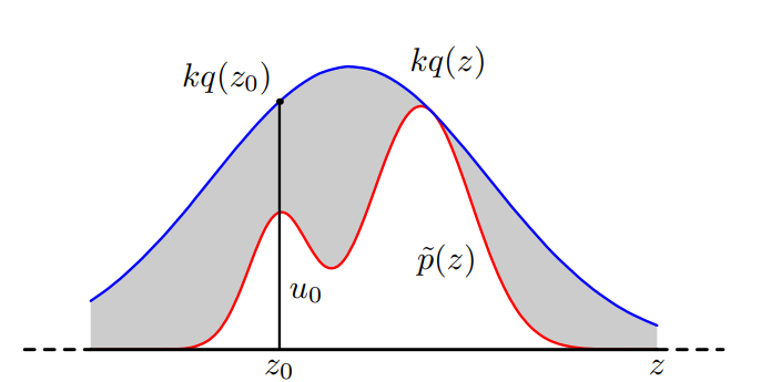
Rejection sampling will not work in high-dimensional case because the acceptance rate will decrease exponentialy with respect to the dimension.

4.2.2. Importance Sampling

Check this book chapter

In Bayesian inference, we are interested in evaluting integral $h(x)$ wrt the posterior distribution $f(x)$.

\[I = E_{f(x)}[h(x)]\]

However, the posterior distribution might not be easy to sample. Instead of using the posterior, we sample from another distribution $g$ to evaluate the integral

\[I = \int h(x) f(x) dx = \int \frac{h(x)f(x)}{g(x)} g(x) dx = E_g [\frac{h(x)f(x)}{g(x)}]\]

Algorithm (importance sampling) We can simluate this by sampling $X_i \sim g$ and estimate

\[\hat{I} = \frac{1}{N} \sum_i \frac{h(X_i)f(X_i)} {g(X_i)}\]

$\hat{I}$ is an unbiased estimator of $I$.

\[E\hat{I} = E_{X} [\frac{h(X)f(X)}{g(X)}] = \int \frac{h(x)f(x)}{g(x)} g(x) dx = I\]

It converges to $I$ almost surely by SLLN

\[\hat{I} \to I\]

This estimator's variance is

\[\sigma_g = \frac{1}{n} \int \frac{h(x)^2 f(x)^2}{g(x)} dx - \mu^2 = \int \frac{(h(x)f(x) - \mu g(x))^2}{g(x)} dx\]

which suggests a good estimator should be

\[g(x) \propto h(x)f(x)\]

approximation of partition function

One example of application is to estimate partition function, let $p(x) = f(x)/Z$ and $q(x)$ be the proposal function

\[Z = \int f(x) dx = \int \frac{f(x)}{q(x)} q(x) dx = E_q[\frac{f(x)}{q(x)}] = \frac{1}{N} \sum_i \frac{f(x_i)}{q(x_i)}\]

Algorithm (self-normalizing importance sampling) If we only know the density up to a constant $f(x) = f_0(x)C_0$ and $g(x) = g_0(x)C_1$, we can still apply the importance sampling using

\[\hat{I} = \frac{\sum h(X_i) w(X_i)}{\sum w(X_i)}\]

where $w(X) = f_0(X) / g_0(X)$.

This still converges to $I$ almost surely by applying SLLN to nominator and denominator separately.

when to use importance sampling

$f(x)$ is difficult to sample from, but can be evaluated up to the constant factor
$g(x)$ is easy to sample and evaluate
we can choose $g(x)$ to be high with $h(x)f(x)$

4.3. Metropolis-Hasting Algorithm

This youtube is very clear explaining the idea here

Let $f(x)$ be the (maybe unnormalized) target density, $x^{(j)}$ be a current value, and $q(x|x^{(j)})$ be a proposal distribution, then

First sample from

\[x^* \sim q(x | x^{(j)})\]

Calculate the acceptance probability

\[\rho(x^{(j)}, x^*) = \min \{ 1, \frac{f(x^*)q(x^{(j)}|x^*)}{f(x^{(j)})q(x^{*}|x^{(j)})} \}\]

Set $x^{(j+1)} = x^*$ with probability $\rho$, otherwise keep the same $x^{(j)}$

Note the sequence $x^{(j)}$ is not independent

Algorithm (random-walk Metropolis) When the proposal distribution is symmetric $q(x | x^{(j)}) = q(x^{(j)} | x)$, then it can be simplified to

\[\rho(x^{(j)}, x^*) = \min \{1, \frac{f(x^*)}{f(x^{(j)})} \}\]

Algorithm (independent Metropolis-Hasting) another simplification is to use $q(x | x^{(j)}) = q(x)$

property (probability, convergence in distribution)

\[x^{(j)} \to X\]

where $X \sim f(x)$

property (expectation, convergence in distribution)

\[\frac{1}{J} \sum_{j=1}^J h(x^{(j)} \to E_f[h(X)] = \int_{\mathcal{X}} h(x) f(x)dx\]

4.4. Gibbs Sampling

Gibbs Sampling is a special case of Metropolis-Hastings algorithms

Consider the distribution $p(z)=p(z_1, ..., z_m)$ from which we wish to sample and we have some initial state.

Each step of the Gibbs sampling is to replce the value of one of the variables $x_i$ conditioned on the existing values of remaining variables:

\[z_i \sim p(z_i | z_1, ..., z_{i-1}, z_{i+1}, ..., z_m)\]

This is repeated for all variables $i$, and repeated for $T$ steps.

5. Approximate Methods

Consider the intractable posterior $p(\theta | \mathcal{D})$

\[p(\theta | \mathcal{D}) = \frac{p(\mathcal{D} | \theta)p(\theta)}{p(\mathcal{D})} = \frac{1}{Z} h(\theta)\]

where $Z=p(\mathcal{D})$ is intractable, the goal is to approximate both $Z$ and posterior $p(\theta | \mathcal{D})$

5.1. Evidence Approximation

Evidence approximation is also known as empirical bayes or Type-2 maximum likelihood.

it may be viewed as an approximation to a fully Bayesian treatment of a hierarchical model wherein the parameters at the highest level of the hierarchy are set to their most likely values, instead of being integrated out.

For example, we can maximize wrt to the hyperparameter $\alpha$ suppose the posterior is sharply peaked around its mode

\[p(\mathcal{D}) = \int p(\mathcal{D} | \alpha) p(\alpha) d\alpha \sim p(\mathcal{D} | \hat{\alpha})\]

where $\hat{\alpha}$ is the mode of posterior $p(\alpha | \mathcal{D})$

5.2. Laplace Approximation

Laplace approximation is used for reasonably well-behaved functions such that most of their mass concentrated in a small region.

\[I(t) = \int \exp({-Nh(x)}) dx\]

After applying the Taylor expansion, we obtained

\[I(N) = \exp(-Nh(\hat{x}))\sqrt{2\pi} \sigma N^{-1/2}\]

where $\sigma^2 = 1/h_2(\hat{x})$ and $\hat{x} = \text{argmin}_x h(x)$

In the multivariate case, the approximation becomes

\[I(N) = \exp(-Nh(\hat{x}))\sqrt{2\pi}^{d/2} |\Sigma|^{1/2} N^{-d/2}\]

where $\Sigma = (D^2h(\hat{x}))^{-1}$ is the inverse of Hessian of $h$ evaluated at $\hat{x}$

Laplace approximation is to approximate this uni-modal distribution with a normal density function.

5.2.1. Marginal Likelihood Approximation

Using the Taylor-expansion around MAP

\[\log h(\theta) = h(\theta_{MAP}) - \frac{1}{2} (\theta - \theta_{MAP})^T \Lambda (\theta - \theta_{MAP})\]

where

\[\theta_{MAP} = \text{argmax} \log p(\theta | \mathcal{D}) = \text{argmax} \log h(\theta)\]

and

\[\Lambda = - \nabla^2 \log h(\theta) |_{\theta_{MAP}}\]

Then we can approximate

\[Z \sim \exp(\log h(\theta_{MAP})) \int \exp(- \frac{1}{2} (\theta - \theta_{MAP})^T \Lambda (\theta - \theta_{MAP})) = h(\theta_{MAP}) \frac{(2\pi)^{d/2}}{(\det \Lambda)^{1/2}}\]

and

\[p(\theta | \mathcal{D}) = h(\theta)/Z \sim \frac{(\det \Lambda)^{1/2}}{(2\pi)^{d/2}} \exp(- \frac{1}{2} (\theta - \theta_{MAP})^T \Lambda (\theta - \theta_{MAP}))\]

5.2.2. BIC

The Bayesian information criterion1 score tries to minimize the impact of the prior as much as possible, therefore, $\theta_{MAP}$ is replaced with $\theta_{ML}$

\[\log p(\mathcal{D}) = \log P(X| \hat{\theta}_{ML}) - (d/2)\log N\]

Note that there is no prior $\pi(\theta)$ in this estimate, so it is clearly not a Bayesian procedure.

5.3. Evidence Lowerbound (ELBO)

Consider the simplest case where the dataset only has one data point: $\mathcal{D} = \{ X \}$. then Evidence $\log p(X)$ can be lower bounded:

\[\log p(X) = \log \int p(X,Z) dZ = \log \int p(X,Z) \frac{q(Z)}{q(Z)} dZ = \log E_{Z \sim q} [\frac{p(X,Z)}{q(Z)}] \geq E_{Z \sim q} \log [\frac{p(X,Z)}{q(Z)}]\]

where the RHS is called evidence lowerbound (ELBO):

\[\text{ELBO} = \mathcal{L}(q, \theta) = E_{Z \sim q(Z)} [\log \frac{p(X,Z|\theta)}{q(Z)}]\]

Another interpretation is $\text{evidence}$ can be decomposed into $\text{ELBO}$ and the KL divergence betwen $q(Z)$ and $p(Z|X)$:

For any choice of $q(Z)$, we have

\[\ln p(X|\theta) = \text{ELBO} + \text{KL}(q(Z) || p(Z|X))\]

This is easy to derive by adding KL and ELBO:

\[E_{Z \sim q} [\log \frac{p(X,Z|\theta)}{q(Z)}] + E_{Z \sim q} [\log \frac{q(Z)}{P(Z|X)}] = E_{Z \sim q} \log p(X) = \log p(X)\]

ELBO is used in both EM algorithm and Variational Inference.

In EM algorithm: we want to find $\theta$ to maximize the evidence $\log p(X; \theta)$

\[\hat{\theta} = \text{maximize}_\theta \log p(X; \theta)\]

In Variational Inference, we want to approximate the posterior $p(Z|X)$.

5.4. Contrastive Divergence

The partition function is usually intractable, so it is difficult to compute the gradient, contrastive divergence (CD) is an approach to estimate the gradient of partition function using (1 cycle) MCMC.

We first rewrite the NLL loss as

\[- \frac{\partial \log P(X)}{\partial \theta} = \frac{\partial \log Z(\theta)}{\partial \theta} - \frac{1}{K}\sum_i \frac{\partial \log f(x_i; \theta)}{\partial \theta}\]

The second term is trivial, the first term can be rewritten as follows: (this derivation can be seen as a special case of gradient estimation)

\[\begin{aligned}\frac{\partial \log Z(\theta)}{\partial \theta} &= \frac{1}{Z(\theta)} \frac{\partial Z(\theta)}{\partial \theta} \\ &=\frac{1}{Z(\theta)} \frac{\partial }{\partial \theta} \int f(x; \theta) dx \\ &=\frac{1}{Z(\theta)} \int \frac{\partial f(x; \theta)}{\partial \theta} dx \\ &=\frac{1}{Z(\theta)} \int f(x;\theta) \frac{\partial \log f(x; \theta)}{\partial \theta} dx \\ &= \int p(x;\theta) \frac{\partial \log f(x; \theta)}{\partial \theta} dx \\ &= \langle \frac{\partial \log f(x; \theta)}{\partial \theta} \rangle_{p(x; \theta)} \\ \end{aligned}\]

where the expectation can be down using sample from MCMC. Empirically, Hinton has found that even 1 cycle of MCMC is sufficient for the algorithm to converge to the ML answer.

with this assumption

\[\begin{aligned} - \frac{\partial \log P(X)}{\partial \theta} &=& \langle \frac{\partial \log f(x; \theta)}{\partial \theta} \rangle_{X^1} - \langle \frac{\partial \log f(x; \theta)}{\partial \theta} \rangle_{X^0}\end{aligned}\]

5.5. Score Matching

This note is a very good summary of score matching of the paper

Model (score matching) Again, consider the situation where we want to train a probabilsitic model

\[p(x | \theta) = \frac{q(x; \theta)}{Z}\]

where $q$ can be evaluated but $Z$ is unknown.

Taking the derivative with respect to $x$, we obtained the equality of score function (note the standard definition of score function in statistics is the derivative wrt to the parameter)

\[\nabla_x \log p(x | \theta) = \nabla_x \log q(x; \theta)\]

$Z$ disappears because it does not depend on $x$. Let us define the score function $\psi(x; \theta)$

\[\psi(x; \theta) = \nabla_x \log p(x | \theta)\]

and $\psi_d(x)$ be the unknown true score function, we would like to match score function between $\psi$ and $\psi_d$

\[J(\theta) = \frac{1}{2} \int p_d(x) \| \psi(x; \theta) - \psi_d(x) \|^2 dx\]

The intuition of this loss function is that if the score function match, we might expect the underlying distribution also matches.

The original paper has a proof that if the true model is within this parameteric model, then minimizing this loss is equivalent of MLE.

To solve this loss, we rewrite it as

\[J(\theta) = \int p_d(x) \sum_i^N [ \partial_i \psi_i(x; \theta) + \frac{1}{2} \psi_{d,i}(x; \theta)^2] dx + const\]

where $\partial_i \psi_{i}(x; \theta) = \frac{\partial \psi_i(x; \theta)}{\partial x_i}$

5.6. Noise Contrastive Estimation

NCE is another model to provide estimation principle to the unnormalized mode. It considers $Z$ as part of the parameter and minimizes a loss function.

Model (NCE loss, noise contrastive estimation)

Let $f(x; \alpha)$ be an un-normalized model (i.e: $p(x; \theta) = f(x; \alpha)/Z(\alpha)$), we consider $Z$ as a parameter and optimize wrt $\theta = (\alpha, c)$ where $c = -\log Z$ and $\log p$ becomes tractable

\[\log p(x; \theta) = \log f(x; \theta) + c\]

Consider another noise distribution $\tilde{x} \sim q(x)$ and define the log odds $l(x)= \log \frac{p_\theta(x)}{q(x)}$, we optimizes the cross-entropy loss

\[\mathcal{L} = \frac{1}{N}\sum_i \log \sigma(l(x_i)) + \log (1- \sigma(l(\tilde{x}_i))\]

Under some conditions, it can be shown this estimator $\hat{\theta}_T$ is consistent: $\hat{\theta}_T \to \theta^*$ in probability. For details about this estimator, check sec 2.3 in the paper.

5.7. Maximum Mean Discrepancy

5.8. Variational Inference

Check Chapter 10 Approximate Inference in PRML and this paper

This is a very good blog in Japanese

The idea behind Variational Inference is to first posit a family of densities and then to find the member of that family which is close to the target. Closeness is measured by Kullback-Leibler divergence. Unlike MCMC approach (probabilistic and exact scheme), Variational Inference is a deterministic approximation scheme.

We first specify a family $\mathcal{Q}$ over latent variables $Z$. Each distribution $Q(Z)$ is an candidate to approximate the exact conditional $P(Z|X)$. We want to find the best one by solving the following optimization problem

\[Q^*(Z) = \text{argmin}_{Q \in \mathcal{Q}} \mathcal{D}[Q(Z) || P(Z|X)]\]

5.8.1. Mean-Field Variational Family

One family commonly used to approximate posterior is the mean-field variational family or factorized distributions

\[Q(Z) = \prod_i Q_i(Z_i)\]

To optimize wrt to this family, we can use the coordinate ascent to optimize each coordinate $Z_j$ everytime, it will lead to a local minimum

\[q^*_j(Z_j) \propto \exp \{ E_{-j} [\log p(Z_j | Z_{-j}, X)] \}\]

5.9. Approximate Bayesian Computation (ABC)

6. Reference

[1] Murphy, Kevin P. Machine learning: a probabilistic perspective. MIT press, 2012.

[2] PRML

[3] Larry's SML book chapter

[4] Michael Jordan's Stat 260 lecture note