0x432 Model
- 1. Statistical Language Model
- 2. Syntax
- 3. Semantics
- 4. Topic Model
- 5. Statistical Machine Translation
- 6. Reference
This page summarizes classical statistical based approaches.
1. Statistical Language Model
Mostly n-gram based language models
1.1. Concepts
Maximum Likelihood Estimator
MLE does not work in practice because of sparseness Backoff Backoff assigns probability with n-1 gram if n-gram is not seen in the training set
1.2. Models
Major models are as follows:
LM (Witten-Bell) LM (Good Turing)
without tear
LM (Jelinek-Mercer) interpolation
LM (Kneser-Ney Smoothing) high order is to use count-based probability with absolute discount
low order is to use the fertility context as the backoff smoothing
Stupid Backoff
1.3. Tools
[1] provides a very good tutorial for efficient implementation
SRILM Tutorial
ARPA format How backoff is estimated in srilm
// compute ppl
ngram -lm corpus.arpa -ppl test_corpus.txt
MSRLM numerator, denominator of normalization are delayed until query. Therefore costs more CPU time for querying. [1] memory-mapping implementation IRSLTM Kenlm data
Google 1 Trillion n-gram (2006) Implementations bit packing: if unigram is less than 1M, trigram can be packed into a 64bit long long by using index of 20 bit for each word rank: store the rank of counting instead of the count themselves
2. Syntax
2.1. Constituent Tree Parsing
2.1.1. CFG
Ambiguities
- coordination ambiguity: CFG cannot enforce agreement in the context. (e.g: koalas eat leaves and (barks))
- prepositional phrase attachment ambiguity (e.g: I saw a girl (with a telescope))
Solution is to use PCFG to score all the derivations to encode how plausible they are
2.1.2. PCFG
2.1.2.1. Estimation
ML Estimation
smoothing is helpful
2.2. Parsing
2.2.1. CKY
complexity is \(O(n^3 |R|)\) where \(n\) is the number of words and \(|R|\) is the number of rules in the grammar
2.2.1.1. Horizontal Expansion
2.2.1.2. Vertical Expansion
2.3. Discriminative Rerankings
generate top-k candidates from the previous parser and rerank them with discriminative reranking might be helpful
Features Classifiers
3. Semantics
3.1. Information Extraction
3.1.1. Relation Extraction
Task (Relation Extraction) Relation Extraction is a task to find an classify semantic relations among the text entities such as: child-of, is-a, part-of and etc.
The text entities can be detected by, for example, name entity recognition.
3.1.2. Algorithms
Algorithm (Hearst patterns) The earlist and still common algorithm is using lexico-syntactic pattern matchings, proposed by Hearst in 1992.
The advantage is it has high-precision, but it has low-recall and takes lot of work.
For example, to recognize hyponym/hypernym, we can use the following patterns \(\(NP_0 \text{ such as } NP_1\)\)
implies the following semantics
Algorithm (supervised training) use whatever classifier you like to. If it is a feature-based classification, the feature can be word feature (bag of words), named entity feature or syntactic feature.
Algorithm (semi supervised) Take some known relations and use these to filter more sentences from unlabeled data, then use those new sentences to train classifier and extract relations with high confidence score, and repeat...
3.1.2.1. Relation dataset
Here is a list of some datasets for relation extraction tasks.
- Wikipedia
- Wordnet
- Freebase
- DBpedia
- TACRED
- SemEval
3.2. Dependency Parsing
3.2.1. Transition-based
3.2.2. Graph-based
4. Topic Model
4.1. Latent Semantic Analysis (LSA)
Apply SVD to term-document matrix, then approximate with low rank matrix
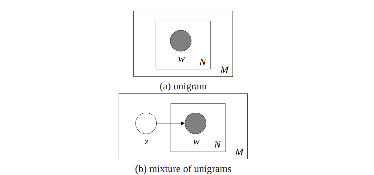
4.2. Mixture of Unigram
Under the unigram model, the word of every document are drawn from an independently from a single multinomial dist4ribution
This is obviously too simple, a
Model (mixture of unigram)
Each model is first generated by choosing a topic \(z\) and then generating \(N\) words independently from the conditional multinomial \(p(w|z)\), the probability of a doc is
4.3. Probabilistic LSA (pLSA)
Document label \(d\) and a word \(w_n\) are conditionally independent given un unobserved topic \(z\)

4.4. Latent Dirichlet Analysis (LDA)
Model (Latent Dirichlet Analysis) Latent Dirichlet allocation (LDA) is a generative probabilistic model of a corpus
The pLSA model is equivalent to LDA under a uniform Dirichlet prior distribution
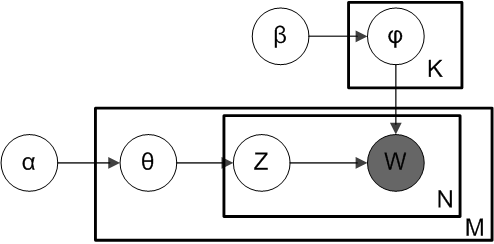
The PGM is the following where "plates" are replicates. Only word \(w\) are observable variables, other are latent variables
- \(M\): number of docs
- \(N\): number of words in a doc
- \(K\): number of topics
- \(\alpha\): Dirichilet prior per doc topic
- \(\beta\): Dirichilet prior per word topic
- \(\varphi_{k}\) is the word distribution for topic k
- \(\theta\): topic distribution for a doc
- \(z\): topic for the a word in a doc
- \(w\): word
4.4.1. Generation
The generative process is
- choose \(\theta_i \sim Dir(\alpha)\) where \(i \in \{ 1, ..., M \}\)
- choose \(\varphi_k \sim Dir(\beta)\) where \(k \in \{ 1, ..., K \}\)
- For each word \(i\) in each doc \(j\)
- Choose a topic \(z_{i,j} \sim Multinomial(\theta_i)\)
- Choose a word \(w_{i,j} \sim Multinomial(\varphi_{z_{i,j}})\)
4.4.2. Inference
The original paper proposes using the Variational Bayes to approximate posterior, other probable approaches are MCMC (e.g.: Gibbs sampling)
5. Statistical Machine Translation
To get translate a Foreign sentence \(f\) into English sentence \(\mathbf{e}\). Two fundamental approaches exist.
- direct model \(argmax_{\mathbf{e}} P(\mathbf{e} | \mathbf{f})\)
- noisy channel model \(argmax_{\mathbf{e}} P(\mathbf{f} | \mathbf{e}) P(\mathbf{e})\)
5.1. Word Model
Suppose \(\mathbf{a}, \mathbf{f}, \mathbf{e}\) denote alignment, Foreign sentence, English sentence respectivelly. Word based model optimize the model \(\theta\) with the alignment model (if noisy channel model) as follows
5.1.1. IBM Model 1
IBM model 1 is the simplest word model with the assumption that \(P(a_j=i | \mathbf{e})\) is constant. It models the joint probability of \(\mathbf{a}, \mathbf{f}\) as follows:
The first term on the right side is the emission probability, the second term is the alignment probability. The alignment probability \(P(a_j | f_j, \mathbf{e}; \theta)\) can be further decomposed as follows. The alignment is estimated in the expectation step.
The translation model is optimized in the maximization step
5.2. Phrase Model
6. Reference
[1] Foundations of Statistical Natural Language Processing