0x375 Search Engine
- 1. Foundation
- 2. Index
- 3. Ranking
- 4. Neural Model
- 5. Search Log
- 6. Personalization
- 7. Federated Search
- 8. Enterprise Search
- 9. Search Log Analysis
- 10. Reference
This note was my lecture notes from CMU 11-642 search engine
1. Foundation
1.1. Exact-Match Retrieval
1.2. Best Match Retrieval
In the Exact-Match retrieval, each document is either matched or unmatched. In the Best-Match model, each document matched to some extent and we retrieve a ranked list of documents. The Exact Match retrieval and Best Match retrieval can be combined for example
Lucene ClassicSimilarity
Lucene's ClassicSimilarity using two steps:
- use a Boolean query to form a set of documents
- use the Best-Match vector space algorithm to rank the documents
1.2.1. Vector Space Model
Suppose the documents can be represented as a vector in vector space, we can then measure the similarity between them using cosine similarity
The problem is how to create the vector, in general, the vector should consider three points
- Document Term weight: importance of the term in the document
- Coolection Term weight: importance of the term in the collection (terms that occur a lot in the collection is useless)
- Length normalization: compensate for varying document length
There are many variants depending on the choice of tf, idf
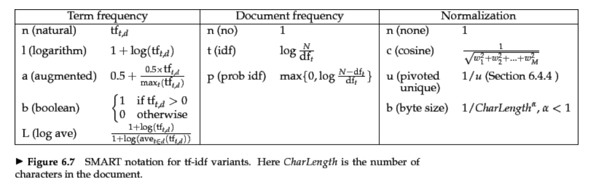
One popular choice is the lnc-ltc model
Model (lnc.ltc) The standard tf-idf model where the tf function is \(\log(tf)+1\), idf function is \(\log(N/df)\) and idf is only applied to the query part. lnc is the notation for document, ltc is the notation for the query, see the table above for their meanings.
where to put idf
In lnc.ltc, idf is applied to the query side. However, difference systems can put it on either or both sides of query and document. For example, Lucene's ClassicSimilarity put it on both sides. It looks there are no theories under it.
Model (Lucene ClassicSimilarity) the vector space model is
- The first term is query-independent document weight (e.g: PageRank)
- The second term is how many query terms matched \(d\)
- The 3rd one is defined as
Notice it is different from the previous lnc.ltc.
BM25 is another related model. According to Lucene documentation, BM25 is superior to the classic similarity model
Model (Okapi BM25) BM25 is a kind of tf idf, tf is saturating function, ranging from 0 to 1, doclen is taken into consideration (longer doc are difficult to saturate) as follows, idf is \(log(N-df+0.5/df)\)
putting them together, we get
1.2.2. Latent Semantic Indexing
Read section 18.4 of IR book
We use SVD to construct low-rank approximation of the term-document matrix \(C\) by taking top-\(k\) singular vector spaces
For a query vector \(q\), we can transform it into the same space \(q_k\) by
The SVD cost is very expensive, so it might not be very practical to use LSI. Additionally, adding new document to the corpus would require recomputing the SVD.
1.2.3. Evaluation
Cranfield Methodology
- documents
- information need
- relevance judgment
- metrics
- comparison of methods
Relevance Feedback can a better query be created automatically ? use user judgement to expand query *10 -20 is good, 100 - 200 is great. if few documents are judged, results are highly variable
disadvantage:
- instable
- not consistent
Pseudo relevance feedback unsupervised machine learning
-
- asume top N (like 50) docs are relevant as positive training data.
-
- apply a relevance feedback algorithm to weight term
-
- expand query
initial and final query can be run on different corpora
Feedback in vector space
- Rocchio algoirthm
- relvant document vector and - non-relevant document vector to query vector
feedback in okapi
- give every term in relevant docs a weight by qtf*RSJ weight
feedback in Indri
- like rocchio
- expansion can loss focus
1.2.4. Document Representation
1.2.4.1. Controlled vocabulary
The library of Alexandria, examples: pubmed, reuters
advantages - browse and search - high recall
disadvantages:
- coverage vs detail tradeoff
1.2.4.2. Free-text, full-text
- free-text: use selected terms from the document
- full-text: use all terms
2. Index
2.1. Index Construction
process:
- each processor receives a part of documents and build an inverted list in its memory
- each processor write inverted list into disks
- inverted list get merged (very fast, because they are usually sorted)
document - documents are usually in large chunks containing lots of documents (to save space probably for inode) - 10 million websites is 250G
2.2. Inverted List
three types:
- binary: df and docid
- frequency: df and docid and tf (term frequency in each docid)
- positional: df, docid, tf and locs (location of all tf counts)
implementation:
- only need integers, field can be guessed from integer.
2.2.1. Compression
- motivation: IO speed is slower than CPU.
- effect: 10 to 15 percent of original size
Delta gap encoding:
- store the difference between docid, locs
- this is to make integer small (skewed distribution)
- stemming also helps
Variable Byte encoding:
- encode integer with variable bytes.
- use the most significant bit as a flag.
2.2.2. Optimization
skip list:
- add skip list to inverted list
- number of skip list is sqrt(df).
- purpose: reduce IO and computation
(top docs) champion lists:
- select best documents in inverted list
- faster but lower recall
how to construct
- select by tf, pagerank
- can be sorted by tf or doc id
- if sort by doc_id, may require multiple lists of different lengths
- if sort by tf, support read variable amount of list
multiple inverted lists perterm
- use two inverted lists. one has locs and one does not have
2.3. Forward Indexes
- map doc to term lists (like labels in kaldi), and field range
- can be constructed in parallel with inverted list
- forward indexes store the indexed form of a document
- the location of every term in in index (term id, location)
implementation:
- indri: create a local stem vocab and use local vocab id
2.4. Large-scale Index
stats:
- google crawl 20B pages/day in 2013
- ave page size: 37k
- ave inlink for any page: 1k
- index size is 20 per of the raw text size
- document size: 1000TB
- Index: 200TB -> 10,000 dollar
2.4.1. Distributed Indexes
- index is divided into partitions (shards)
- each shard will process a set of documents
- 1 machine has 2 disk of 4TB, 40 machines to hold 320TB index
2.4.1.1. Document Partitioned Index
how to distribute corpus into different shards ?
- random assignment: balances query traffic across partitions, simple update policy
- source-based assignment: better compression of inverted lists
2.4.1.2. Tired Indexes
- high-value pages and low-value pages
- search from low-value tiers if top tier is not good enough
- how to select ? page rank, click thourhg, short URL, low spam scores
advantage:
- lower the cost
- improve search quality
- go to tier 2: mistake ? exact match ? rare ?
2.4.2. Cache
*check result cache -> check inverted list cache -> normal search
2.4.2.1. cache query result
- 25 query are over 1% of the traffic. 64% occur once before
- 20 to 30 per of queries had been seen recently
- 30 per of search queries match a cache, at some point increase cache does not help
- half of query is seen before
- saturates faster
- check first
2.4.2.2. cache inverted lists
- cache query term inverted lists
- which to cache: high frequent in query log
- do not have long inverted lists
- score = qtf divided by df
- typically the list cache size is a few GB
- check second
2.4.3. Index Construction
2.4.3.1. MapReduce
simple approach:
- map document into (term docid) list. Each is a parser indexer
- shuffle term into its corresponding processor
- reducer convert streams of keys into streams of inverted lists
advanced approach:
- build partial inverted list instead of (t,d) -> fewer data shuffle
- sort inside map task -> easier for reducer to sort
- build different apple inverted for each partition (partitioned indexes)
2.5. Indexing and Priors
2.5.1. Inverted File Managmenet
static File:
-
no updates is easier because no empty space between inverted lists
-
when delete a document, just add its id to a delete list
2.5.2. Indri Index Components
term dictinoariy: - Indri has two term dictionary, one for frequent term, and one for rare terms
inverted files - one for terms - one for fields
2.5.3. Prior
2.5.3.1. Query-Independent Evidence
- does not appear in query
- page rank, spam score, difficulty
- linear combine all vector space to get vector space score
2.6. Document Structure
2.6.1. Fields
- independent fields
- no hierarchical structure
- vocab independent
- fields can provide '''different representation''' of '''the same information'''
- some fields are better '''evidence''' (inlink)
- some fields are '''verbose''' (body)
How to handle fields
- fields stand for multiple Representations of Meaning
- fields can be used to provide different representations of the same information
Vector Space
- how to retrieve -> weight score for each field
- vector space solution(lnc.ltc): treat F bow, and add scores
BM25F
- problem: BM25 is using saturating tf do not reflect frequent term appearances.
- solution:
- 1)create a big BoW by weighting tf in different fields
- 2)weight tf term with constant in different field
characteristics:
- one '''global''' vocab and global idf
- tf is field specific tuned
Indri
- wand: '''independent prob'''
- wsum: combine '''different way of estimating the same prob'''
2.6.2. Hierarchical Document Structure
characteristics:
- elements are related to others
- a term occur in all elems containing it
- goal is to retrieve doc or elem
Indri
Jelinek-Mercer smoothing:
- the smoothing term is expanded to linearly combine elems containing them
- aggregation can be done during indexing or querying
Aggregation
- combine '''inverted lists'''
- disadvantage: cannot rank
Combination
- combine '''score'''
- preserve inlink info while combining scores
- sum-element op(max, and, sum): combine children scores into parent score
3. Ranking
3.1. Learning to Rank
Pointwise
- x to category or score
bad:
- less accurate than others
- ignore ordinal category, scores are arbitrary
Pairwise \(x_1 > x_2\)
Listwise: use softmax as a generating model
3.2. Authority Metric
3.2.1. PageRank
- query independent and topic independent
- random walk between teleport or follow link
- page rank is like vote, popular pages have more votes
variation: - how to handle new pages - how to handle link farms
3.2.2. Topic-Sensitive PageRank
- during indexing, each page is assigned to a topic
- teleportation is allowed to pages within a topic
- each document has a topic distribution
- teleportation is based on topic distribution
- TSPR is linear weighted by topic specific TSPR
3.2.3. HITS
- hyperlink-induced topic search
- only compute score for a local graph, not the entire web
- root set: query specific doc set
- base set: root set + links-to and links-from
algorithms: - each page in base set has a hub score and authority score - hub score is computed from authority score - authority is computed from hub score - repeat
bad:
- easier to spam than PageRank
- runtime cost
good: to find communities
3.3. Diversity
issue:
- there are multiple '''user intents''' or interpretations
- each intent has multiple '''tasks'''
- trade-off: robustness vs relevance
solution:
- rerank top n to create diverse ranking
3.3.1. Metric
Precision-IA@k (Intent-Aware):
- P@k weighted by intent prob distribution
- document satisfying multiple intent get good score
alpha-NDCG:
- original NDCG is the sum of relevance score discounted by ranking
- gain: weighted gain of different intent discounted by relvance sum
3.3.2. Implicit
MMR(Maximum Marginal Relevance):
- decrease doc score when they are similar with current doc in rankings
- sim can be lnc.ltc or JS divergence.
LeToR for diversification:
- add similarity feature with highly ranked docs to LeToR
- similarity feature: text similarity, link similarity, URL similarity
- scores for highly ranked docs can be combined by average, min, max
- relational-ListMLE is to add sim feature to softmax
3.3.3. Explicit
two types of intents:
- navigational
- informational
two types of topics:
- ambiguous: jordan
- faceted: obama family tree
search engine provide suggested and related queries
xQuAD
- select a new doc that cover new uncovered intents
- prefer documents that satisfy multiple intents
PM2
- compute qt (vote) for each intent
- pick up doc based on intent qt
- update s (score)
- PM2 can pick up rare intents
- it maintain proportion of each intent
4. Neural Model
repersentation based
4.1. Representation based Model
- encode q into vec
- encode d into vec
- compute cos
4.1.1. DSSM
Term Vector Layer:
- vocab: 500k terms
- each word is represetned by a vector of trigrams
Word Hashing Layer:
- 500K -> 30k trigram
- low collision rate
Multi-layer nonliear project:
- 300 -> 300 -> 128 (semantic feature)
4.2. Interaction based Model
4.2.1. DRMM
- compute cos score between all q_i and d_j
- bin values for cos and distinguish '''exact matching''' bin
- compute histograms (count matches, normalized count, log of count)
- gated score by applying idf
4.3. Kernel based Model
4.3.1. K-NRM
5. Search Log
find similar users
- build pseudo documents with (user, query)
- body is the category for top n docs of each query
- apply similarity metric to cluster
- what: check topics
- who: demographic info
- how: how they search
Segmentation
- delta time: check time stamp
- common term: same session if has same term
- rewrite class: same session if query get modified
feature based:
- temporal
- edit distance
- query log co-occurrence
- prisma
Mission and Goals
- '''information''' is a single, well-defined goal
- '''mission''' is a set of related information needs
two tasks:
- boundary task: whether a pair consecutive query is same goal or mission
- same task: whether a pair of query is same goal or mission
5.1. Query Suggestion
- return the last query in the session
pseudo documents
- create pseudo docs and apply retireval model
- title: last query
- body: previous query
co-occurrence stats:
- set1: frequent query has q as a substring
- set2: frequent query following q
Query Intent
how to create query intent cluster
- expand: identify most common reformulation and its reformation
- filter: connect q1 and q2 if same d get clicked, and remove empty nodes
- cluster: find groups with same intent using random walk
- popularity estimate: random walk
- name: name the group with the highest score query
5.2. Click Model
- click models represent behavior as a sequence of observed and hidden events
- E: examined
- A: attracted(a measure of snippet quality)
- C: clicked
- S: satisfied
Random Click Model (RCM)
- each doc (url) is equally clicked, not accurate
Ranked-based Click Through Model (RCTR)
- one of Click-Through Rate (CTR)
- click prob depends on its rank
Document-based Click Through Mdodel (DCTR)
- CTR on query and doc
- prone to overfit
Position based Model
- click depends on examination and attractiveness
Cascade Model
- examines the SERP from top to bottom until a relevant model
others
- time spent on SERP item
- scrolling
- eye movement
5.3. Within-session Learning
people gain domain knowledge through exposure and interaction
two types:
- procedural knowledge: how to do
- declarative: what is
6. Personalization
three approaches:
- topic-based personalization
- long-term vs short-term personalization
- personalization for typical/atypical information need
6.1. Topic-based Personalization
three component:
- representation
- learning
- ranking
evaluation:
- data: ODP
- metric: mean reciprocal rank(MRR)
- micro-averaged F1 on ODP
- macro-averaged F1 on ODP(class distribution is ignored in macro)
- good effect on acronyms (because ambiguous)
6.2. Long-term vs Short-term
three types of information:
- historic: information acquired over a long period of time(historic)
- session: information from current search session
- aggregate: historic + session
Query-Doc-User features:
- cosine between topic categories of document and view
- cos between topic categories of doc and query
Query features:
- ambiguity measures: click entropy, topic entropy
- difficulty measures:
query
- ambiguity measures: click entropy and topic entropy
- difficulty measures: position in session
methodology: 6+32*3=102
6.3. Personalization for typical and atypical
not complete
7. Federated Search
7.1. Resource Representation
Model:
- BoW: terms and frequencies
- Sample queries: queries that this resource is good for
- sample documents: typical docs from this resource
How to get:
- request via protocol (e.g: STARTS hard to use)
- request relevance
- query-based sampling: submit a query and see results
7.2. Resource Selection
Task: given a query, decide which resources to search
7.2.1. unsupervised methods
- resource ranking problem
- estimate p(r_i|q) and select top k
CORI:
- Content-based methods
- treat each resource as a BoW
- CORI(adapted from BM25)
- common approach is to order by how many relevant doc each resource contains
good: more efficient than ReDDE
bad:
- tends to generate homogeneous results
- miss large, heterogeneous collection
Query-based methods:
rank resources based on the similarity of the query to past queries that the resource matched well
ReDDE:
- voting based on random samples ranking
- better than CORI when the distribution is skewed
- weak bias towrd large collections
- slower
7.2.2. supervised methods
query features:
- boolean: e.g. weather.
- geo feature
- clarity: KL div between top ranked docs and the entire collection
8. Enterprise Search
8.1. Faceted Search
How to:
- Use inverted lists to index facets
- use forward indexes to index facets
- store facets in a relational database
8.2. Query Suggestion
9. Search Log Analysis
query session (search session) is a sequence of query submitted by one unique user within a short time of interval
9.1. Query Suggestion
20% of all searches are unique, 97% of all searches occur less than 10 times
9.1.1. Pseudo Document
For a search trail \((q_1, q_2, ..., q_n)\). Under the assumption \(q_n\) corresponds to the actual user's intent. Create a pseudo document with \(q_n\) as the title, \((q_1, ..., q_{n-1})\) as the body. To get a suggestion, start a new query into this pseudo documents and return the title.
9.1.2. Co-occurrence
Suggestions based on the co-occurrence within the same search session. Its disadvantage is data sparsity and cannot deal with long-tail queries
Rank the suggested query with \(Count(q_s)\) and \(Count(q, q_s)\) where \(Count(q_s)\) is the popularity of suggested query and \(Count(q, q_s)\) is the count of co-occurrence of \(q_s\) follow the user's actual query \(q\) in the search session. looks like Bayesian approach.
10. Reference
[1] CMU 11-642 https://boston.lti.cs.cmu.edu/classes/11-642/
[2] Manning, Christopher D., Prabhakar Raghavan, and Hinrich Schütze. Introduction to information retrieval. Cambridge university press, 2008.