0x412 Bayesian Model
1. Naive Model
Probably the most simple model for supervised learning is to just fit a single parametric distribution to the data, this is much simpler than linear models and nonlinear models.
For a single class, we simply model \(p(x)\) with a simple parameteric distribution, for multiple class, we model it with
where \(y\) is a class, and \(x\) might be discrete or continuous.
These generative models can be used, for example, classification tasks by modeling generative distribution for each class.
1.1. Discrete Model
Fit a parametric discrete model
1.1.1. Multinoulli Naive Bayes Model
The motivation of using Naive Bayes is to reduce the complexity. Consider the model has \(n\) features, each feature is a binary feature. Without any constraints, we would need to model
for every \(i,j\) and this results in around \(O(2^{n+1})\) parameters to estimate, which is usually too expensive.
With naive Bayes assumptions, we can reduce this complexity significantly. It writes the class conditional density of one-dimensional density
The parameters of NB model is small \(O(CD)\) where \(C\) is the number of class, \(D\) is the number of feature, so relatively immune to overfitting.
The joint distribution \(p(x, y)\) is then
And the posterior is
In this binary classification task, the decision boundary is \(p(y=1|x) = p(y=0|x) \implies \log{\frac{p(y=1|x)}{p(y=1|x)} = 0}\)
This simplifies to
1.2. Continuous Model
Fit a parametric continous model
1.2.1. Gaussian Model
1.2.2. Gaussian Discriminant Analysis
This looks to be a bad naming, it is actually a generative classifier.
It fits the Gaussian distribution for each class conditional distribution
1.2.2.1. Quadratic Discriminant Analysis
The most general form is to assume Gaussian distribution without any contraints on \(\mu_c, \Sigma_c\)
This will produce quadratic decision boundary (as its name indicates).
Gaussian Naive Bayes and Linear Discrimnative Analysis are two special forms of QDA.
1.2.2.2. Gaussian Naive Bayes
Gaussian Naive Bayes assumes conditional independence, therefore the off-diagnoal entry of \(\Sigma_c\) will be zero, therefore \(\Sigma_c\) is contrained to be diagonal matrix.
Note that this still can produce quadratic decision boundary. It will produce linear boundary when variance are tied.
1.2.2.3. Linear Discriminative Analysis (LDA)
LDA are using the same covariance matrix.
This produces the linear decision boundary.
2. Latent Variable Models
2.1. Discrete Models
2.1.1. EM Algorithm
EM is an algorithm which is guaranteed to converge to the (local) MLE or MAP
Consider the observed variables are \(X\) and hidden variables or latent variables are \(Z\). The direct optimization of \(p(X|\theta)\) is difficult, but the optimization of the complete data likelihood \(P(X,Z | \theta)\) is easy. \(P(X,Z)\) might belong to exponential family, but \(P(X) = \int P(X,Z) dZ\) is not.
For example, recall \(P(X)=\sum_k \pi_k \mathcal{N}(x|\mu_k, \Sigma_k)\) in GMM is not very tractable, but \(P(X,Z) = \pi_k \mathcal{N}(x|\mu_k, \Sigma_k)\) is tractable
We start from \(\theta_0\) and iteratively repeat E step and M step.
Consider the ELBO formula:
In the E-step, we evaluate \(p(Z|X, \theta_i)\) and set
this will make KL to be 0 and increases the lower bound: left hand is unrelated to q, so right hand is constant, decreasing KL will increase ELBO
Then we formulate the \(\mathcal{Q}(\theta)\) function:
In the M-step, we maximize \(\theta\) with respect to the new \(q(Z)\)
the right hand is written in the complete data form, so it should be easy to optimize
2.1.2. Gaussian Mixture Model
As an example, we derive the EM Algorithm for the Gaussian Mixture Model.
The Prior is
The conditional probability is
Combining them together gives the complete data likelihood:
Taking log yields
In the E-step, we evaluate
and we know
The \(\mathcal{Q}\) function becomes
In the M-step, we maximize them to obtain
where \(N_k = \sum_n \gamma(z_{nk})\)
2.2. Continuous Models
See Chapter 12 of PRML
2.2.1. Probabilistic PCA
The prior over \(z\) is
and the conditional distribution of the observed variable \(x\), conidtioned on the value of the latent variable \(z\) is
3. Bayesian Network
Bayesian Network is the directed graphical model, it provides a skeleton for representing a joint distribution compactly in a factorized way as follows
Note that BN is ambiguous: there are many BNs to represent the same distribution.
3.1. Representation
Local Structures and Independencies
- common parent (B->A, B->C, tail to tail): knowing B decouples A and C
- cascade (A->B->C, head to tail): knowing B decouples A and C
- v-structure (A->C, B->C, head to head): knowing C couples A and B
Definition (independence function \(I\)) Let \(P\) be a distribution over \(X\). We define \(I(P)\) to be the set of independence assertion of the form \(X \perp Y | Z\) that holds in \(P\)
Definition (I-map) A graph \(G\) is i-map of distribution \(P\) if \(I(G) \subseteq I(P)\) (i.e. any independence \(G\) asserts much also hold in \(P\))
Intuitively, it is just means that \(G\) is a consistent expressing graph of the distribution \(P\).
D-separation is a framework to collect independences in the graph.
Criterion (D-separation) a procedure to check independence between nodes given some other nodes. If those nodes are connected after following steps, they are dependent. Otherwise they are independent at least in bayesian network.
- build ancestral graph
- moralize graph (connecting parents of the v-structure)
- remove direction
- remove conditional nodes
There is an equivalence theorem related to the specification of probability distribution
D-separation is sound and "complete" with respect to factorization law
- soundness: If a distribution \(P\) factorizes according to \(G\), then \(I(G) \subseteq I(P)\)
- completeness: For any distribution \(P\) that factorizes overs \(G\), if \(X \perp Y | Z \in I(P)\), then \(dsep_{G}(X; Y | Z)\)
Theorem (equivalence theorem) For a graph \(G\),
- Let \(D_1\) denotes the family of all distributions that satisfy \(I(G)\)
- Let \(D_2\) denotes the family of all distributions that factor according to \(G\) (i.e: \(P(X) = \prod P(X_i | X_{parent})\))
Then
3.2. Naive Bayes
The probability estimation of Naive Bayes tends to be poor when the input \(\mathbf{x}\) have interdependence (which violates the conditional independence assumption). For example, if we repeat the input feature \((x_1, x_1, x_2, x_2, ..., x_n, x_n)\) then the confidence will be increased even the information does not increase
3.3. Markov Model
The easiest way to treat sequential data is to ignore the sequential aspects and treat the observations as i.i.d, which would be too naive. However, it would be impractical to consider a general dependence of future observations on all previous observations.
Model (Markov models) we simplify the dependency relation and assume the future predictions only depend on the most recent observations. In the first order markov model, we have
from it we can derive the joint distribution
Increasing the order of Markov chain would increase the number of parameters. For example, if we have \(K\) discrete states with \(M\)-th order, the parameters are \(K^m(K-1)\), which grows exponentially.
If we want to build models with high dependency, but with limited parameters, we can introduce the latent variables to build state space model.
- When the latent variables are discrete, it is hidden markov model
- When the latent variables (and observed variables) are continuous, it is the linear dynamical system
The joint disbitribution is given by
3.4. HMM
The observed variables in an HMM may be discrete or continous, but the latent variables are discrete. If the latent variable are Gaussian (continuous), then we obtain the linear dynamical system. Both HMM and linear dynamical system are instances of state space model.
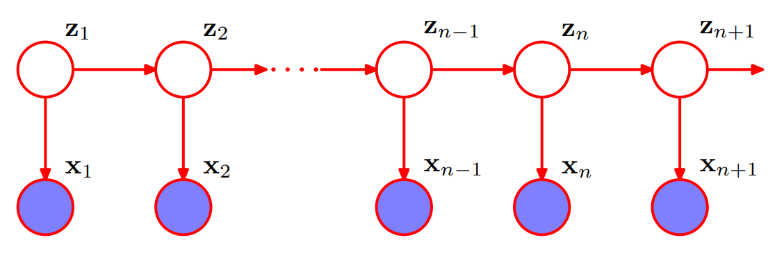
The joint probability distribution over both latent and observed variables is given by
where \(X = \{x_1, ..., x_N \}\) are observed variables, \(Z=\{ z_1, ..., z_N \}\) are latent variables, \(\theta=\{ \pi, A, \phi \}\) are paramters.
The initial probability using \(\pi_k = p(z_{1k} = 1)\) is
The transition using \(A_{jk} = p(z_{nk}=1 | z_{n-1, j}=1)\) is
The emission probability is
HMM has the key conditional independence property that \(z_{n-1}\) and \(z_{n+1}\) are independent given \(z_n\)
However, it allows the observation \(x_n\) to have infinite dependence over all history: any \(x_n, x_m\) are unblocked due to the d-seperation criterion. The predictive distribution \(p(x_{n+1} | x_1, ..., x_n)\) does not exhibit any conditional independence properties, so it depend on all previous observations.
There are three problems in HMM:
- evaluation problem: Given observations \(X\) and model \(\theta\), find its marginal probability \(P(X; \theta)\)
- decoding problem: Given observations \(X\) and model \(\theta\), find the conditional probability of latent states \(P(Z | X; \theta)\)
- learning (inference) problem: Given the observations \(X\), find the model \(\text{argmax}_\theta P(\theta | X)\)
3.4.1. Evaluation
The evaluation problem answers the question: what is the prob that a particular sequence of symbols is produced by a particular model
For evalution problem, we have two methods: forward-algorithm or backward-algorithm
Model (forward-algorithm) We first define the forward probability with \(\alpha(z_n)\)
It has the recursion
and initial condition as
Model (backward-algorithm) Similarly, the backward probability is \(\beta(z_n)\)
It has the recursion
and the initial condition as
Using \(\alpha, \beta\), we can compute the marginal probability for any choice of \(n\)
If we choose \(n=N\), then it is simply
3.4.2. Decoding
First recall the following two problems are not same:
- finding the most probable sequence of latent states
- finding the set of states that are individually the most probable. (which can be solved by running forward-backward)
This can happen, for example, two successive states are most probable themselves, but the transition connecting them is 0.
Given a sequence of symbols (your observations) and a model, what is the most likely sequence of states that produced the sequence \(P(Z | X; \theta)\)
Model (viterbi) For decoding problem, we use the Viterbi algorithm (max-sum algorithm)
3.4.3. Inference
Training problem answers the question: Given a model structure and a set of sequences, find the model that best fits the data.
For inference problem, we have the Baum Welch = forward-backward algorithm
Model (Baum Welch) In addition to the \(\alpha, \beta\), we define two more posteriors variables
Expanding \(p(X|z_n)\), we get
by using d-separation. Combining with the previous formula, we get
3.5. MEMM
See this book chapter
Maximum Entropy Markov Model (MEMM) is a discriminative model using maximum entropy
Notice this is a Markov Model because of the \(\prod P(y_i | y_{i-1})\) structure
There is a labelling bias issue with MEMM, which can be addressed by CRF. The labelling bias is caused by the difference of the normalization: MEMM adopts local variance normalization (i.e: MEMM normalize with \(Z(y_{i-1}, \mathbf{x})\) for every step \(i\)) while CRF adopts global variance normalization (i.e: CRF normalizes \(Z(\mathbf{x})\) globally).
For more details about label bias, see this Awni's blog
3.5.1. Inference
Same as the Logistic Regression
3.5.2. Decoding
Viterbi
3.6. Structure Learning
When the structure is unknown,
This note summarizes some approach to learn the Bayesian graph structure from training data
4. Reference
[1] Bishop, Christopher M. Pattern recognition and machine learning. springer, 2006.
[2] Rosenblatt, Frank. Principles of neurodynamics. perceptrons and the theory of brain mechanisms. No. VG-1196-G-8. Cornell Aeronautical Lab Inc Buffalo NY, 1961.
[3] Minsky, Marvin, and Seymour A. Papert. Perceptrons: An introduction to computational geometry. MIT press, 2017.
[4] Sutton, Charles, and Andrew McCallum. "An introduction to conditional random fields." Foundations and Trends® in Machine Learning 4.4 (2012): 267-373.
[5] CS229 Lecture Note
[6] Mitchell, Tom M. "Machine learning." (1997).