0x531 VAE

The idea behind the latent variable model is to assume a lower-dimensional latent space and the following generative process

\[Z \sim P(Z)\]

\[X \sim P(X|Z)\]

We want to sample from the simple low-dimensional latent space $Z$ easily (e.g: Gaussian), and maximize the evidence function over the dataset $X \sim \mathcal{D}$

\[P(X) = \int P(X|Z; \theta)P(Z)dZ\]

The idea behind the latent variable model is to assume a lower-dimensional latent space and the following generative process

\[Z \sim P(Z)\]

\[X \sim P(X|Z)\]

We want to sample from the simple low-dimensional latent space $Z$ easily (e.g: Gaussian), and maximize the evidence function over the dataset $X \sim \mathcal{D}$

\[P(X) = \int P(X|Z; \theta)P(Z)dZ\]

2.1. Vanilla VAE

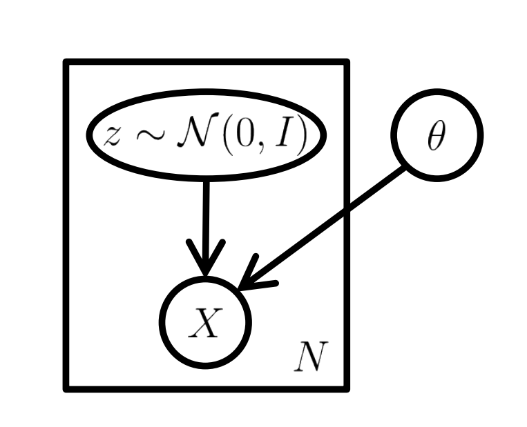
VAE implement this idea with the following modeling

Model ($P(Z)$) the prior in VAE is

\[P(Z) = N(0, I)\]

Note this is a fixed prior in contrast with the VQ-VAE's learnt prior

Model ($P(X|Z)$) likelihood is modeled using a a deep neural network function $f(Z; \theta)$: VAE approximates $X \approx f(Z; \theta)$ and measure $P(X|Z)$ by penalizing using Gaussian distribution

\[P(X|Z; \theta) = N(X | f(Z; \theta), \sigma^2I)\]

if $X$ is discrete, it can other discrete distribution penalty such as Bernouli)

Probabilistic PCA

Recall pPCA is a simplified version of VAE

\[P(Z) = N(Z | 0, I)\]

and likelihoood function $f$ is linear

\[P(X|Z) = N(X | WZ + \mu, \sigma^2I)\]

The graphical model of VAE is

graphical model

The integration of evidence is very expensive,

\[P(X) = \int P(X|Z)P(Z) dZ\]

so we are maximizing the lower bound of evidence (ELBO) instead of the evidence itself

Recall the the standard ELBO form (RHS usually denoted $\mathcal{L}(Q)$) is

\[\log P(X) \geq E_{Z \sim Q}[\log\frac{P(X,Z)}{Q(Z)}]\]

where the right hand expression is the ELBO, ELBO can be further decomposed into two terms

\[ELBO = E_{Z \sim Q} \log \frac{P(X|Z)P(Z)}{Q(Z|X)} = E_{Z \sim Q}[ \log P(X|Z)] - \mathcal{D}[Q(Z|X)||P(Z)]\]

We model $Q(Z|X)$ as

\[Q(Z|X) \sim N(\mu(X), \Sigma(X))\]

wherre $\mu(X), \Sigma(X)$ is implemented using neural network.

Look at the formula again,

\[ELBO = E_{Z \sim Q}[ \log P(X|Z)] - \mathcal{D}[Q(Z|X)||P(Z)]\]

The first term on RHS has a sampling step $z \sim Q$ which cannot backprogate. The training process can be done using the reparametrization trick where we sample $\epsilon \sim N(0, I)$ and transform $\epsilon$ to $z$ (instead of sampling $Z \sim Q$ directly)

\[Z = \mu + \Sigma^{1/2} \epsilon\]

The 2^nd term is simple to compute

\[\mathcal{D}[Q(Z|X)||P(Z)] = KL(N(\mu, \Sigma) || N(0, I)) = \frac{1}{2}(tr(\Sigma) + \mu^T\mu - k -\log\det\Sigma)\]

The likelihood function cannot be exactly calculated, only the lower bound could be provided

2.2. Posterior Collapse

VAE suffers from the posterior collapse problem when the signal from posterior $Q(Z|X)$ is too weak or too noisy, it collapses towards the prior

\[Q(Z|X) \sim P(X)\]

where a subset of $Z$ is not meaninfully used and it matches the uninformative prior

The decoder then starts ignoring it and generate sample without signal from $X$, the reconstructed output becomes independent of $X$

Some works claims this is because of the KL term in the objective,

Most common approaches to solve these are either

change objective
weaken decoder

2.3. Architecture

Model (VAE-GAN) Attach a discriminator after encoder/decoder.

2.4. Loss

Model ($\beta$-VAE) attempts to learn an disentangle distribution with $\beta > 1$

\[E_{Z \sim Q}[ \log P(X|Z)] - \beta KL[Q(Z|X)||P(X)]\]

Another approach to solve the posterior collapse problem

Model ($\delta$-VAE) prevent KL from falling to zero by constraining posterior $Q$ and prior $P$ such that they have a minimum distance $KL > 0$

A trivial choice is to set the Gaussian with a fixed different variance. For a non-trivial sequential model, they use non-correlated $q$ and corelated prior AR(1)

\[P(Z_t | Z_{<t}) = N(Z_t; \alpha Z_{t-1},, \sigma_{\epsilon})\]

There is a minimum distance because one is correlated and the other is not correlated

2.5. Vanilla VQ-VAE (Discrete Model)

Model (VQ-VAE) VQ uses the discrete latent variables instead of the continous one. It has a latent embedding $e \in R^{KD}$ where $K$ is the size of the discrete latent space and $D$ is the hidden dimension.

vqvae

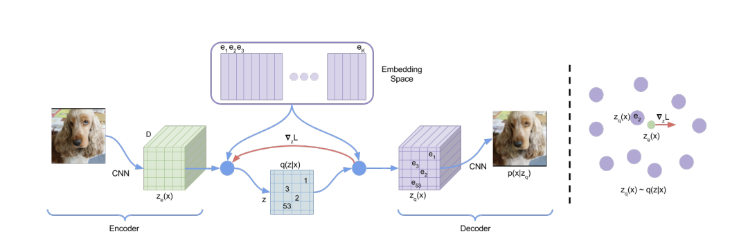
It models the posterior distribution as a deterministic categorical distribution

\[q(Z=k | X) = \begin{cases} 1 \text{ when } k = \text{argmin}_j ||z_e(x) - e_j|| \\ 0 \text{ otherwise} \end{cases}\]

The loss function is

It consists of

reconstruction loss: $\log p(x|z_q(x))$
codebook loss: $\| sg[z_e(x)] - e \|^2$, bringing codebook close to encoder output, can be replaced with EMA (exponential moving average) for stability
commitment loss: $ |z_e(x) - sg[e] |^2$, encourages encoder output to be close to codebook

VAE vs VQ-VAE

VQ-VAE can be seen as a special case of VAE. The KL term in the original VAE disappears by assuming prior $p(z)$ is uniform $p(z=k) = 1/K$ and the proposal distribution $q(Z=k|X)$ is deteterministic:

\[KL[Q(Z|X) || P(Z)] = \sum_{i=1}^K q(z|x) \log \frac{q(z|x)}{p(z)} = q(z=k |x) \log \frac{q(z=k|x)}{p(z=k)} = \log K\]

While training the model, the prior $p(Z)$ is kept constant and uniform $p(z=k)=1/K$,. After training, it can be fit to an autoregressive model over $Z$, so that we can sample using ancestral sampling

In this work, they model the autoregressive latent prior using PixelCNN for image and WaveNet for raw audio

The experiment settings are interesting

Image settings:

128x128x3 -> 32x32x1 (K=512)
43 times reduction

Audio settings:

encoder: 6 convolution with stride 2 and window 4 (K=512)
64 times reduction
decoder: dilated convolutional architecture like the WaveNet decoder

Problems:

The VQVAE also has its own problem, namely, the low codebook usage due to poor codebook initialization.

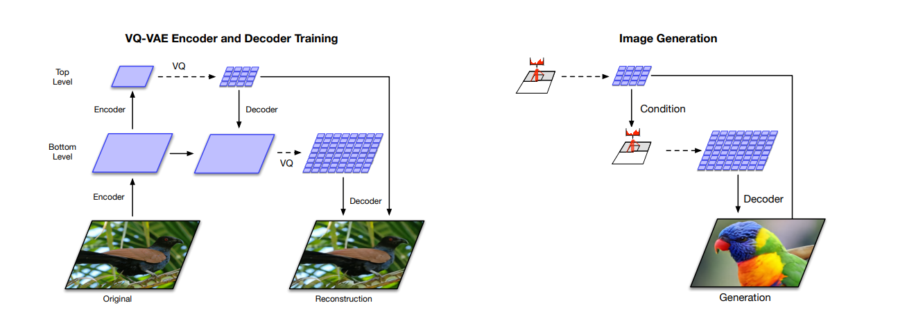
2.6. Hierarchical VQ-VAE

Model (Hierarchical VQ-VAE)

It has a hierarchical latent code

top latent code models global information
bottom latent code, conditioned on the top latent, models local information

256x256 images -> 64x64 (bottom) -> 32x32 (top)

Prior

top prior: PixelCNN + multihead self attention to capture larger receptive field
bottom prior: no self-attention

vqvae2