0x530 Adversarial

Goodfellow's tutorial

Let \(X \in \mathcal{X}\) be the random variable of interest, \(P(X)\) to be its distribution and a training sample \(X_1, ..., X_n\).

We have two main components:

• generator: a map \(g_\theta: \mathcal{Z} \to \mathcal{X}\). It takes an random Guassian noise \(Z\) and generates outputs \(g_\theta(Z)\). Its goal is to choose \(\theta\) such that \(g_\theta(Z)\) is close to \(X\)
• discriminator: a map \(D_w \mathcal{X} \to [0, 1]\). its goal is to assign 1 to samples from the real distribution \(P_X\) and 0 to samples from the generated samples \(P_\theta\)

The parameters are \((\theta, w)\), it can be obtained by solving the min-max problem

\[\min_\theta \max_w E [ \log(D_w(x)) + \log(1-D_w(g_\theta(x))) ]\]

It is equivalent to minimizing the JS divergence

\[\min_\theta JS(P_X \| P_\theta )\]

It means we choose the closest \(P_\theta\) to the target distribution \(P_X\) in the JS divergence

5.1. Problems

5.1.1. Vanishing Gradient

5.1.2. Mode Collapse

5.2. Architecture

Model (DCGAN, deep convolutional GAN) transposed convolution to upsampling

An application of DCGAN (2 dim) to audio generation (1 dim) is WaveGAN

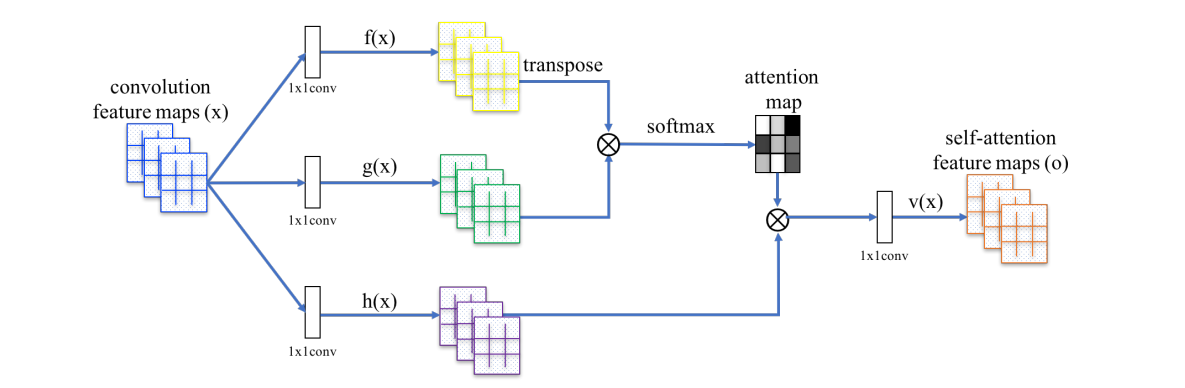
Model (SAGAN, Self-Attention GAN)

Add self-attention to GAN to enable both generator and discriminator to model long-range relation. \(f,g,h\) in the figure is corresponding to \(k,q,v\)

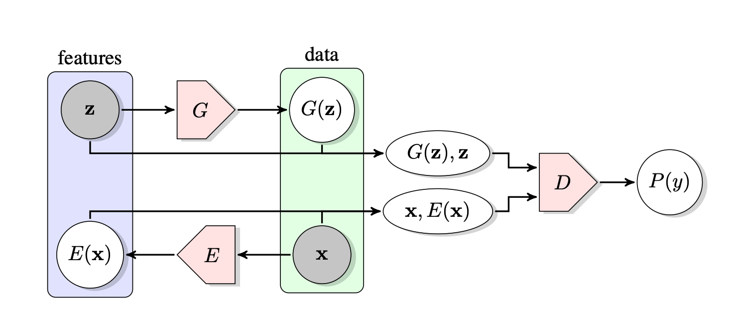
Model (BiGAN) use discriminator to distinguish whether \((x,z)\) is from encoder or decoder

5.3. Representation

Model (Info GAN) Modifies GAN to encourage it to learn meaning representation by maximizing the mutual information between a small subset of noise and the observations.

The input noise vector is decomposed into \(z\): incompressible noise, \(c\), latent code which encode salient semantic features. The goal is to minimize \(I(c; x=G(z,c))\), which is not available because \(P(c|x)\) is unknown.

Instead we lower bound this using an auxiliary distribution \(Q(c|x)\) to approximate \(P(c|x)\)

\[I(c; G(z,c)) \geq E_{x \in G(z, c)} E_{c' \sim P(c|x)} [\log Q(c'|x)] + H(c)\]

By ignoring the second term and rewriting the first term, the lower bound becomes

\[L_I(G,Q) = E_{c \in P(c), x \sim G(z,c)} [\log Q(c|x)]\]

5.4. Loss

Model (spectral normalization) Stabilize the training of dsicriminator by normalize the weight by its spectral norm so that its Lipschitz constant is controlled

\[\bar{W} = W/\sigma(W)\]

Model (WGAN, Wasserstein GAN)

The main points of WGAN is to replace the JS distance to \(L^1\)-Wasserstein distance. because

• Wasserstein distance respects the geometry of underlying distribution
• it captures the distance between two distribution even their support do not intersect

Not intersecting support is common in high dimensional applications where the target distribution lies in a low dimensional manifold

Recall the \(L^1\)-Wasserstein distance is

\[W_1(P_X, P_Y) = \inf_\pi E [ | X - Y | ]\]

where \(\pi\) is any coupling between pair of random variables \((X,Y)\).

It can be shown that the Wasserstein distance \(W_1(P_X, P_{g_\theta})\) is continuous with respect to \(\theta\) if \(g_\theta\) is continous wrt \(\theta\)

To minimze \(W_1(P_X, P_\theta)\), we use the Kantorovich-Rubinstein duality

\[W_1(P_X, P_\theta) = \sup_{\|D \|_L \leq 1} E [D(X) - D(g_\theta(Z))]\]

where the sup is over functions whose Lipschitz constant is less than 1, expanding the entire forms, we get

\[\min_\theta \max_w E [ D(X) - D(g_\theta(Z))]\]

subject to \(\| D \|_L \leq K\)

In practice, the constraint is enforced by constraining the infinity norm of the weights (known as clipping)

tutorials:

• Here is a short introduction to optimal transport
• A good introduction to the WGAN
• a mandarin introduction

Model (WGAN-GP, WGAN + Gradient Penalty)

Model (LS-GAN) use least-square instead of sigmoid cross entropy in discriminator, it can

• generates higher quality
• stable learning process

5.5. Application forcused GAN

Model (Cycle GAN)