0x513 Transformer
- 1. Foundation
- 2. Positional Encoding
- 3. Attention Model
- 4. Low Rank/Kernel Transformer
- 5. Patterns-based Transformer
- 7. Other Variants
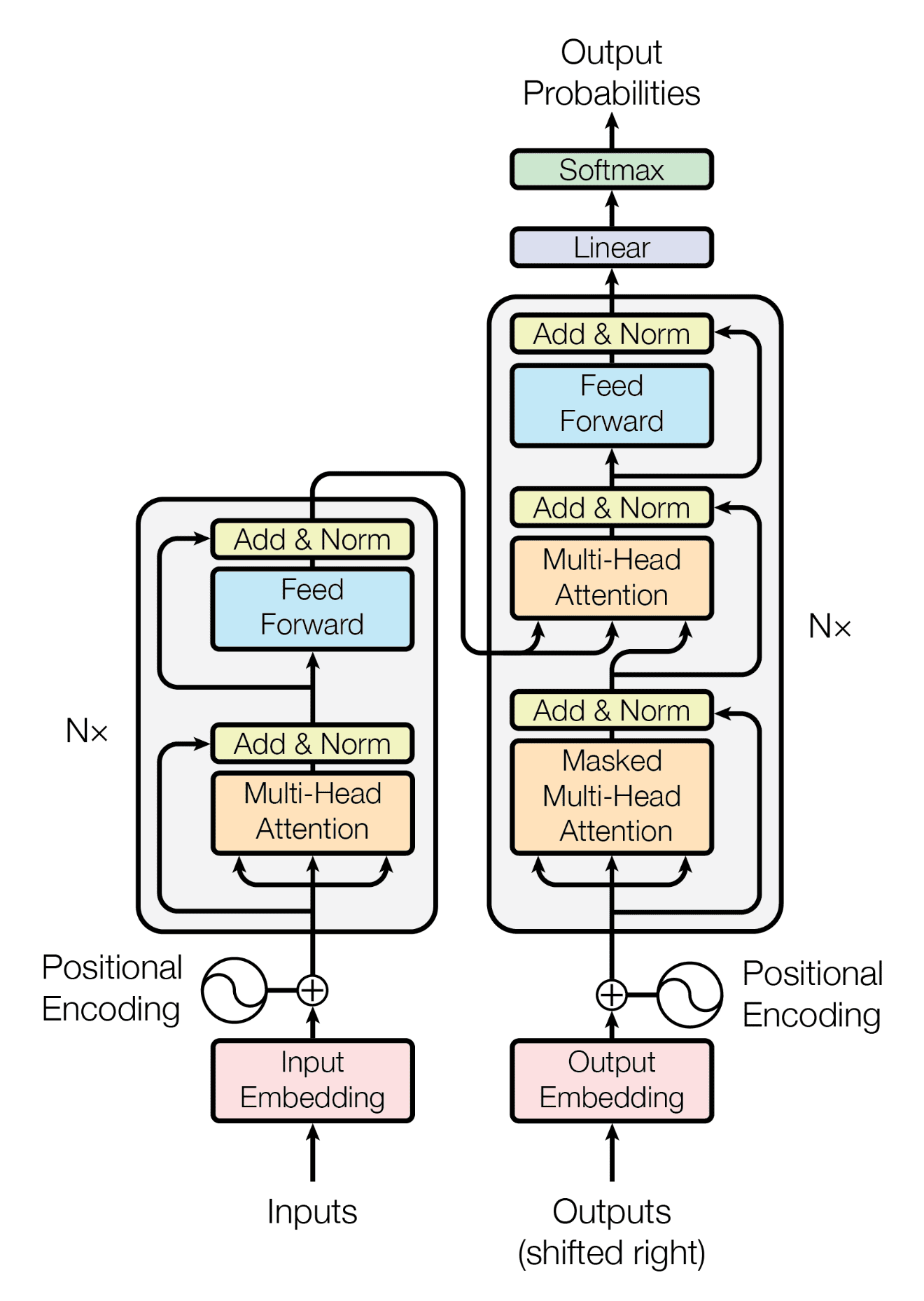
Transformer combines two important concepts:
- recurrent free architecture
- multi-head attention aggregate spacial information across tokens
Many recent transformers are variants of efficient "X-former", see this survey paper
1. Foundation
With the following abbreviations
- B: batch size
- E: embedding size
- L: layer size
- H: number of hidden size
- N: number of heads
- V: vocab size
- T: target sequence length
- S: source sequence length
1.1. Numbers
1.1.1. Paramter Estimation
The total number of parameters are roughly
- embedding layer: \(VE\)
- transformer layer: ~\(L(12E^2)\): out of 12, 4 are from QKVO, 4+4 are from 2 layer feedforward (note that layer norm parameter are ignored)
This gives a good estimation of GPT2's parameter
- 117M tiny: 12 layer + 768 dim + 50257 vocab (~124M)
- 345M small: 24 layer + 1024 dim + 50257 vocab (~353M)
- 762M medium: 36 layer + 1280 dim + 50257 vocab (~758M)
- 1542 large: 48 layer + 1600 dim + 50257 vocab (~1554M)
1.1.2. Computing Estimation
1.1.3. Memory Estimation
See this blog post
Model Memory Roughly in the inference, only 4 bytes per parameter is used, in the training 16 bytes (param + grad + 2 optimizer state) per parameter are used if not optimized.
The following detailed reference is from the Huggingface's transformer doc
Model Weights:
- 4 bytes * number of parameters for fp32 training
- 6 bytes * number of parameters for mixed precision training (maintains a model in fp32 and one in fp16 in memory)
Optimizer States:
- 8 bytes * number of parameters for normal AdamW (maintains 2 states)
- 2 bytes * number of parameters for 8-bit AdamW optimizers like bitsandbytes
- 4 bytes * number of parameters for optimizers like SGD with momentum (maintains only 1 state)
Gradients
- 4 bytes * number of parameters for either fp32 or mixed precision training (gradients are always kept in fp32)
Activation Memory Without any optimization, it will be roughly the following
- input+output: \(2BTV\) one-hot vector input/output (can be ignored compare the next)
- transformer: ~\(L \times BT(14H + TN)\)
Also see this paper for some activation analysis under 16bit
2. Positional Encoding
See this blog for some intuition
Model (sinusoidal positional encoding) The original transformer is using the sinusoidal positional encoding
where \(\omega_0\) is \(1/10000\), this resembles the binary representation of position integer
- where the LSB bit is alternating fast (sinusoidal position embedding has the fastest frequency \(\omega_0^{2i/d_{model}} = 1\) when \(i=0\))
- But higher bits is alternating slowly (higher position has slower frequency, e.g. 1/10000)
Another characterstics is the relative positioning is easier because there exists a linear transformation (rotation matrix) to connect \(e(t)\) and \(e(t+k)\) for any \(k\).
Sinusoidal position encoding has symmetric distance which decays with time.
The original PE is deterministic, however, there are several learnable choices for the positional encoding.
Model (absolute positional encoding) learns \(p_i \in R^d\) for each position and uses \(w_i + p_i\) as input. In the self attention, energy is computed as
Model(relative positional encoding) relative encoding \(a_{j-i}\) is learned for every self-attention layer
3. Attention Model
3.1. Attention
The problem of a standard sequence-based encoder/decoder is we cannot cram all information into a single hidden vector. Instead of a single vector, we can store more information in variable-size vectors.
Model (attention)
- Use query vector (from decoder state) and key vectors (from encoder state).
- For each query, key pair, we calculate a weight and weights are normalized with softmax.
- Weights are multiplied with a value vector to obtain the target hidden vector.
Weight \(a(q,k)\) can be obtained using different attention functions, for example:
multilayer perception (Bahdanau 2015)
bilinear (Luong 2015)
dot product (Luong 2015)
scaled dot product (Vaswani 2017, attention paper)
As mentioned in the attention paper, this scaling is to make sure variance is 1 under the assumption \(q=(q_1, ..., q_d), k=(k_1, ..., k_d)\) has independent mean 0 var 1 distribution. Recall the variance of indepedent multiplication from the probability note
3.2. self-attention
Self-attention allows each element in the sequence to attend other elements, to make a more context sensitive encoding. For example, in the translation task, the in English might be translated to le, la, les in French depending on the target noun. An attention from the to the target noun will make it more context sensitive.
Model (self-attention) The self-attention transforms an embedding \((T,H)\) into another embedding \((T,H)\). Shape is invariant under the self-attention transformation
- Input: \((T,H)\)
- Output: \((T,H)\)
- Params: \(W_q, W_k, W_v \in R^{(H,H)}\)
where \(T\) is the sequence length, \(H\) is the hidden size, and \(W_q, W_k, W_v\) are weight matrix.
We first created three matrix \(Q, K, V\), meaning query, key and value.
Next, we query each token to all keys in the sentence and compute their similarity matrix \(S\) normalized by hidden size (scaled dot product)
The \((i,j)\) element is the similarity between token \(i\) and \(j\), each row is normalized by the softmax.
Finally, the similarity is multiplied by the value matrix to get the new embedding \(SV \in R^{(T,H)}\)
Model (multi-head self-attention) Multihead attention use multiple head for self-attention
4. Low Rank/Kernel Transformer
5. Patterns-based Transformer
Check this survey
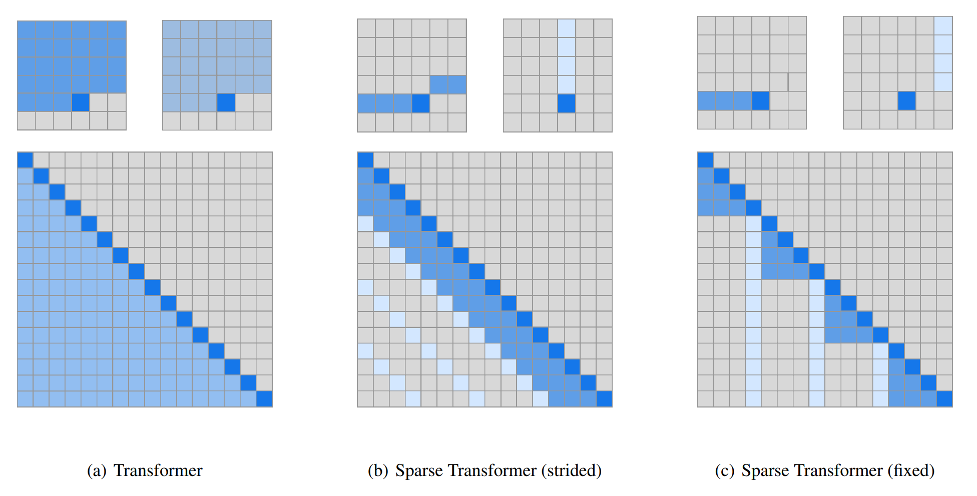
Standard Transformer cannot process long sequences due to the quandratic complexity \(O(T^2)\) of self-attention, both time and memory complexity. For example, BERT can only handle 512 tokens. Instead of the standard global attention, the following models try to circumvent this issue by using restricted attention
Model (sparse transformer) it introduces two sparse self-attention patterns:
- stride pattern: capture periodic structure
- fixed pattern: specific cells summarize previous locations and propagate them into all future cells
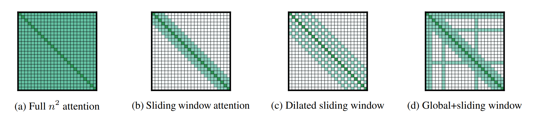
Model (Longformer) Longformer’s attention mechanism is a combination of the following two
- windowed local-context self-attention
- dilated sliding window
- an end task motivated global attention that encodes inductive bias about the task.
Model (BigBird) use global token (e.g: CLS) and sparse attention
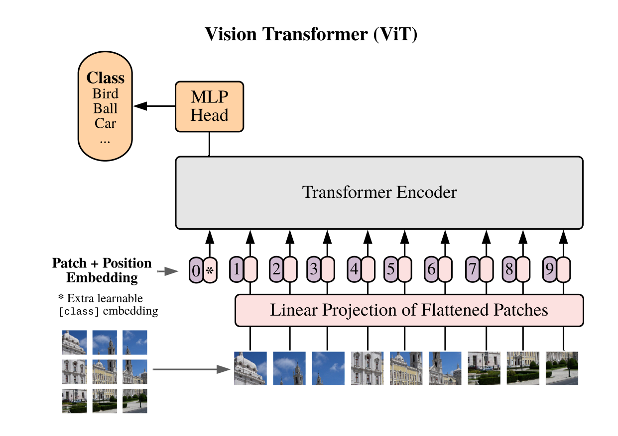
1.2. Vision Transformer
Model (vision transformer, vit) use transformer instead of cnn
- images is splitted into patches, 224x224 images is splitted into 16x16 patches. each patch has 14x14 (196 dim), each patch is like a word-embedding, there are 16x16 words on total.
- a learnable embedding (like the BERT's class token) is prepend before the patch sequence.
- pos embedding (trainable 1d pos embedding) are added
- can be used as a self-supervised training with masked patch prediction.
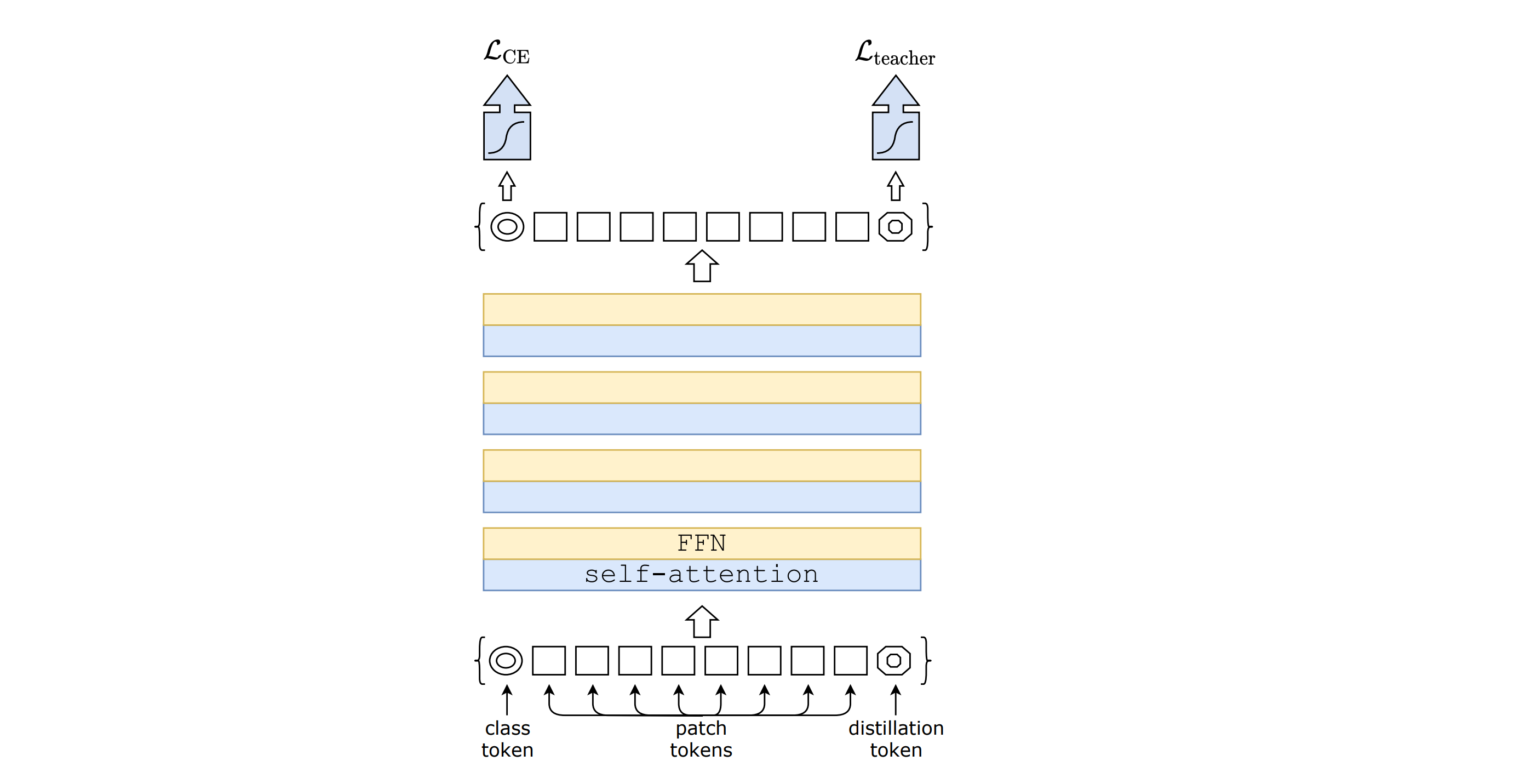
Model (DeiT, data-efficient image transformer) distill information from a teacher ViT model
1.2.1. Hierarchical Model
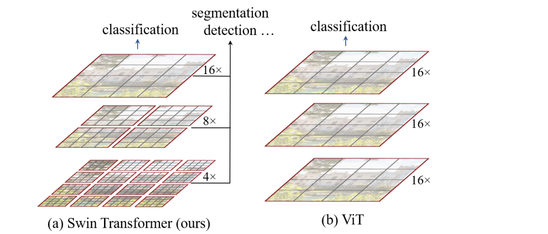
Model (swin transformer)
Swin Transformer block
- attention is limited to a local window
- those window will shifted across layers
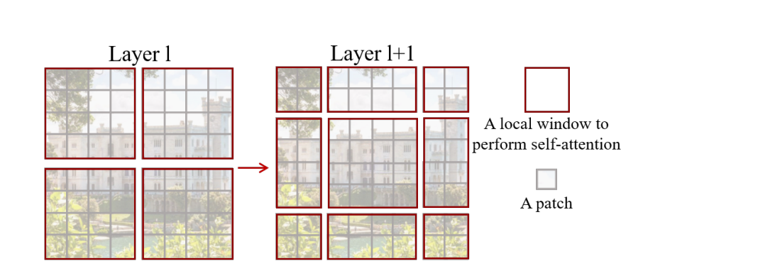
those blocks are forming stages hierarchy in which a layer merging neighbor patches
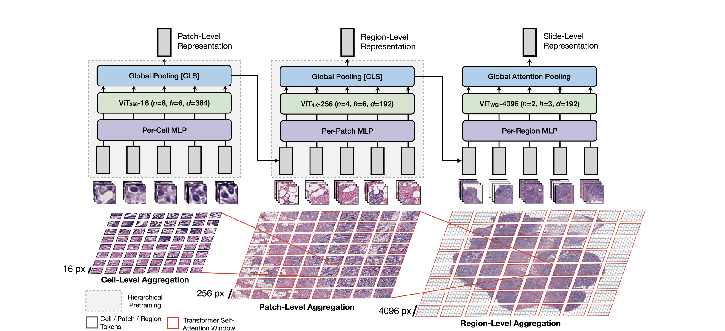
Model (HIPT, Hierarchical Image Pyramid Transformer) High resolution tranformer model using hierarchical model
7. Other Variants
Model (Primer) has smaller training cost than the original for autoregressive LM.